Model-based Reasoning and the Control of Process Plants
Abstract
In addition to stabilizing feedback control, safe and economic operation of industrial process plants requires discrete-event type logic control, for example automatic control sequences, interlocking and protections. A lot of complex routine reasoning is involved in the design and verification & validation (V&V) of such automatics. Similar reasoning is required in action planning and fault diagnosis during plant operation. Much of the required reasoning is so straightforward that it could be accomplished by a computer if only there were plant models which allow versatile mechanised problem solving. Such plant models and related inference algorithms are the main subject of this report.
Applying model-based reasoning in the design and V&V of plant automatics and in action planning during plant operation is discussed. A prototype tool called ISIR (interval simulation and reasoning) for model-based reasoning is presented. The approach is based on the principles of QSIM, an algorithm for qualitative simulation, and it is implemented in constraint logic programming language CLP(). ISIR is applied to the verification and synthesis of a simple discrete-event control strategy of a continuous process, to a power plant feed-water system and to various standard examples from the qualitative simulation literature.
The emphasis of the report is on presenting the principles of the approach, and on demonstrating its potential applications. Because constraint logic programming and the programming techniques developed in this work may be utilized as such programming examples and most of the ISIR-algorithm are discussed in detail. The results are well-defined principles, a prototype implementation, some demonstrations and ideas for the specification of a general-purpose tool.
Keywords: process plant control, discrete-event control, qualitative modelling, qsim, constraint logic programming, deep knowledge.
Keywords:
model-based reasoning, discrete-event control, verification, validation, constraint logic programming, industrial process plants, qualitative modelling, qsim
Reformatted 2018:
I found the tex-files of my dissertation (the last but version of it) from almost 25 years back. I could not resist the temptation to try to convert it to html with latexml. It worked OK. Except the figures, which I had to scan from an print, because the files were lost from the backup.
Also small parts of the text had disappeared. I tried to find the errors and fill in the missing text, but there may still be sentences breaking in the middle.
If the equations do not seem nice on your browser, please try the the pdf-version
Acknowledgements
I want to thank my supervisor Paavo Uronen for his efficient support in getting this work finished.
I want to acknowledge the staff of OECD Halden Reactor Project in Halden, Norway for fruitful co-operation. Especially I want to thank Terje Sivertsen for his interest and valuable help.
The research activities in the Electrical Engineering Laboratory of the Technical Research Centre of Finland (from the beginning of 1994 VTT Automation) had a significant impact on the direction of my work. I want to thank the staff for giving me such a course which I am still happy with. I also want to thank everybody in VTT Automation for the relaxed but also goal-oriented atmosphere.
I want to thank Dr. Kuipers and his colleagues for providing me the QSIM-algorithm and all the advice on using it.
I want to thank all those who made it possible for me to use CLP(). Especially I want to thank Roland Yap for valuable help in solving my constraint logic programming problems.
I want to thank Dr. Sandro Bologna from ENEA, Italy for his encouraging interest and the inspiring discussions we have had.
I want to thank Heikki Tuominen for providing me the understanding on mathematical logic and logic programming when I was starting this work.
I want to thank OECD Halden Reactor Project, Finnish Ministry of Trade and Industry and Imatran Voima foundation for the funding, which made this work possible.
My wife Maija and my daughters Annastiina and Ilona deserve special praise for patiently letting me work also late in the evenings as even now when writing these lines.
Contents:
- 1 INTRODUCTION
- 2 CONTROLLING DYNAMIC SYSTEMS
- 3 CONSTRAINT LOGIC PROGRAMMING
- 4 THE ISIR-ALGORITHM
- 5 A POWER PLANT FEEDWATER SYSTEM
- 6 A CONTINUOUS STIRRED TANK REACTOR
- 7 OSCILLATING SYSTEMS
- 8 DISCUSSION
- 9 CONCLUSIONS
- A ABOUT PROLOG
1 INTRODUCTION
The motivation for this research arose from the following observations on operating and control of industrial process plants:
-
•
Traditional control engineering concentrates on continuous-time feedback control while for the design of automatics — automatic control sequences, interlocking, protections etc. — there exist no mature tools although they constitute an essential part of a typical control system;
-
•
Due to increasingly strict requirements on the operation of industrial process plants and due to the tendency to increase the level of automation the current practices to design control systems may not be sufficient in the future;
-
•
Stricter requirements on plant operation and the development of information technology increase the interest in sophisticated operator support systems. However, there is no mature generic method of implementing support for example for action planning;
-
•
Knowledge based techniques are widely proposed to be applied on problems related to process plant operation. However, mainly heuristic expert knowledge represented as rules is utilized while most of the knowledge needed in plant operation can be obtained from plant design documents;
-
•
Formal methods are promoted for software development and verification and validation (V&V). However, formal development is often based on software requirement specifications which are considered a significant source of errors. To avoid errors originating from software requirements specifications the formal methods should be extended to cover also the environment of the software, for example the process plant to be controlled or monitored.
Plant operation, control system design, autonomous control, constructing knowledge-based design and operator support systems and formal development of safety-critical control and monitoring systems have common denominators:
-
•
They all require a plant model which can be used to solve a large variety of different types of problems;
-
•
The systems addressed have both continuous and discrete dynamics;
-
•
Often the knowledge must be on an abstraction level higher than real-valued functions; generalisations of the plant behaviour rather than particular solutions are needed.
-
•
Uncertainty and incomplete knowledge must be handled properly.
Always when addressing process plant control or monitoring the conventional control engineering the perspective illustrated in Fig. 1 should be adopted.
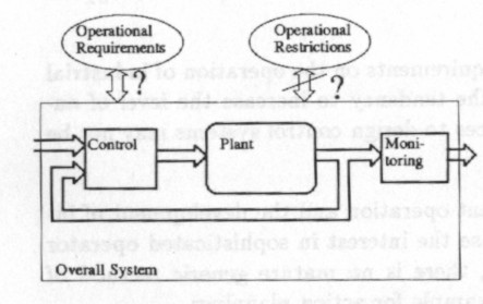
This problem description can be applied to designing plant automatics, to specifying embedded system software requirements, to constructing a knowledge-based system to control or to monitor the plant, and to operator support systems.
In this work techniques are developed which allow the use of supporting computers in solving control and monitoring problems which can be characterized as follows:
- Plant:
-
The plant dynamics can be modelled accurately enough with ordinary differential equations. Optionally some parts of the plant can be modelled as a state automaton.
Sometimes only rough quantitative knowledge or even only qualitative knowledge of the plant is available.
- Control:
-
Control tasks accomplished mainly with sequences of discrete actions driven by discrete events are addressed. Start-up, shutdown, batch process control etc. imply such control tasks. Autonomous control with the requirement to recover from faults and failures require this type of control as well.
Tuning of e.g. PID-controllers is not addressed but it is assumed that continuous-time feedback control works according to its specifications.
- Monitoring:
-
There is a tendency to design alarm systems so that they take into account the operational state of the plant. This work provides some possibilities to guarantee that the alarm system reacts on all the illegal conditions and only on them.
Fault diagnosis, finding an explanation why the plant does not work properly, can be seen as a dual problem to plant control.
- Operational requirements:
-
Operational requirements describe the desired operation of the plant, the goal of operation, as specified by the designer of the plant. The specification may contain quantitative performance criteria but this work addresses problems where a significant part of the desired operations is described with logic clauses and state automata.
- Operational restrictions:
-
Operational restrictions complement the operational requirements by specifying undesired operation. It is typically specified with logic conditions that should never become true. They may give limits never to be exceeded, and they may tell something about illegal order of operating pumps and valves.
1.1 CONTENTS OF THIS REPORT
In the following introduction plant control in general is briefly discussed. The use and the design of discrete-event control is discussed to present the central field of this work. Then links to software engineering and developing knowledge-based systems are indicated.
Computer aided design is discussed to determine the role of computerised tools in control system design.
Section 2 gives a brief introduction on existing analysis and synthesis tools for dynamic systems are discussed. References to qualitative reasoning literature relevant to this work are presented. Finally, different ways to represent the knowledge available and needed in control system design and plant operation are discussed.
Section 3 discusses constraint logic programming. The emphasis is on examples demonstrating the algorithms and programming techniques applied in implementing ISIR.
Section 4 presents the ISIR-algorithm. After examples on applying ISIR on the verification and design of discrete-event control systems it is shown how subtasks in model-based reasoning are dealt with when implementing ISIR. It is also shown how the ISIR-models can be applied in conventional simulation and dynamic optimisation and it is discussed how to integrate these techniques into the basic ISIR-algorithm. Support for model generation is briefly discussed.
Section 5 demonstrates how to construct an ISIR-model of a power plant feedwater system.
Sections 6 and 7 demonstrate the analysis of a behaviour of a continuous stirred tank reactor and oscillating systems. The former is an example to test the ability of a qualitative reasoning tool to discover significantly different system behaviours. Analysis of the oscillating systems is another test to find the limits of a tool.
Section 8 discusses the strengths and the limitations of ISIR and the work needed to make it into a practical general-purpose tool.
Appendix A gives an overview on prolog and constraint logic programming in CLP().
1.2 CONTROLLING PROCESS PLANTS
A control task can be determined by
-
the description of the system to be controlled, i.e. the plant model;
-
the specification of the operational restrictions, and the ‘cost’ of operation;
-
the specification of the goal of operation.
Some kinds of plant models are used in designing plant control strategies and in supporting plant operation. There are different types of plant subsystems and different types of problems to be solved requiring different types of models. Sometimes a rough mental model supported by plant P&I-diagrams is sufficient, sometimes the model must be suitable for formal mathematical manipulation.
The objective is to determine a control strategy which meets the goal and minimises the cost of operation without violating the operational restrictions like safety margins. The goal of the control can be given as the boundaries of the desired state of the plant or as performance criteria to be maximised. There are also operational restrictions given strictly as logic conditions on symbolic values like ‘when = running then it must be = open’, etc. The goal of operation may give some explicit constraints on the inputs, but mainly it constrains the outputs of the system. The goal is not given as a single state or a trend curve but as a performance criterion to be maximised and/or as a set of logic conditions to be satisfied. The control strategy must determine the inputs which result in a behaviour satisfying the requirements. The inputs must be determined as a function of time and/or as a function of the plant state.
Control tasks form a hierarchic structure. On the lowest level single components like pumps are controlled. A large pump driven by an electric motor requires quite a complex control logic.
Stabilizing chemical and physical processes or making them follow given references is on the next level in the hierarchy. In addition to the above, unit control includes initiating and stopping the processes and taking them from one mode of operation into another. In batch production these tasks may constitute the major part of the control system.
The use of the process units must be co-ordinated, the raw materials and intermediate products must be transferred between process units and storages in the plant. The processes must be provided with the resources, for example cooling, needed during the process. All this type of scheduling and solving the routing problems is on the next level in the control hierarchy.
Depending on the type of the control requirements and on the type of the plant subprocess to be controlled, different kinds of control strategies are applied. Continuous time feedback control is used to keep given process outputs at given reference values, optimisation is applied to determine optimal operation region or optimal trajectory to change the states of continuous time subsystems, discrete-event automatics are used to change the plant mode of operation.
Both closed-loop and open-loop control must be dealt with. All on-line control requires feedback — closed-loop control — due to uncertainties in the process models and external inputs11Feedback in a PID control loop is very different from the feedback employed in an automatic control sequence to e.g. start up a plant.
It is not sufficient to find a sequence of control actions which accomplishes a state change in a simulator. A general, robust control strategy insensitive to external disturbances must be determined. This can be applied on a wide range of operation. Such strategies cannot be implemented without feedback.
In action planning and control system design open-loop scenario generation to predict all the alternative behaviours and the extreme bounds of those plant behaviours is needed.
1.3 DISCRETE-EVENT CONTROL
In addition to stabilization, reference following and determining optimal control for continuous processes, it is necessary to start up and shut down complex process plants and change their mode of operation through applying mainly discrete control actions. Discrete-event control or logic control is also used for example to control the phases of a chemical batch process according to a given recipe, to recover from exceptional situations after a component malfunction, in partial plant shutdown for maintenance, to control processes having complex discrete dynamics and only simple continuous-time subprocesses, and in safety systems and interlocking. The control actions are taken by the operator or by plant automatics consisting of automatic control sequences, interlocks and protections.
Because of possible failures and large disturbances it is difficult to foresee in advance all the situations which can be encountered. Therefore, the control system must be able to determine the controls on-line i.e. feedback control is necessary. PID-controller keeping the output in its reference and an automatic control sequence to start up a plant are both feedback controllers but for the latter there are no systematic design methods.
Stricter requirements on the efficiency, raw material and energy saving as well as a need for flexible production require new types of plants, new ways to operate them, higher level of automation and more sophisticated operator support systems. Monitoring, supervisory control and diagnosis tasks earlier handled manually must be automated or the operators must be provided with computerised operator support systems to accomplish the tasks optimally.
The higher the level of automation, the more important the role of the automatics, and the more complex the automatics grow. Considering highly autonomous operation shows clearly the importance of automatics and potential benefits of some sort of mechanised reasoning.
1.3.1 Designing discrete-event control
The theory of traditional control engineering has been successfully applied in solving a wide range of industrial control problems in the continuous-time domain. However, industrial process control is not only determining the optimal value for a real-valued control signal but also opening and closing valves, starting and stopping pumps, switching on and off stabilizing controllers, etc. This kind of control is executed by discrete-event control systems which are called also automatics in this report. Many high-level control tasks are implemented using discrete-event control rather than any kind of continuous time control. This is mainly because of the nature of the task but also because discrete-event control gives good enough results while requiring less accurate models and less computing capacity.
Automatic control sequences have a discrete set of possible states, their input is a set of discrete (often binary) signals and output is a set of discrete control actions. State transitions are triggered by input signals. Interlocking and protection are implemented as a separate part of a discrete-event control system. Interlocking prevents the automatics or the operator from taking certain control actions in situations where they might take the plant in an unsafe state. Protections take the plant from an unsafe to a safe state, for example by shutting it down. Documentation standard for discrete-event control systems is presented in [24].
Discrete-event control is commonly used in implementing control tasks where many of the functional requirements can be specified by conditions telling what is acceptable and what is unacceptable rather than as a criterion to be minimised. Designing discrete-event control strategies does not typically require accurate plant models but much of the design can be based on rough qualitative knowledge. More important than reproducing the actual behaviour with high accuracy is to characterise the essential events and other properties of the behaviour in a way that can be made efficient use of. General qualitative characteristics of the behaviour are important, not exact particular predictions of the behaviour. Only final tuning of the time delays and of the threshold values of taking some actions require more exact quantitative information.
Designing discrete-event control systems requires that many different situations be considered. One of the difficulties is to detect all the qualitatively different alternative behaviours of the plant and to determine all the necessary preconditions of a successful control action and to notice all the possible consequences of a control action. Possible errors in the design are incomplete exception handling, unforeseen side-effects in the co-operation of various pieces of automatics, etc. Many errors are due to various mindlocks caused by the complexity of the behaviour of the overall system.
Some questions that should be asked during the design:
-
Do the interlocks prevent unsafe operation in every situation?
-
Do the interlocks prevent normal operation in some situation?
-
Do the interlocks prevent necessary corrective actions in some abnormal situation for example after a component failure?
-
Can the control sequence be initiated in every situation it is needed?
-
Do the preconditions of the sequence prevent initiating it in every case it cannot or should not be executed?
-
Can the sequence be executed under all the anticipated external inputs and disturbances?
-
Do the automatics function properly in all the plant states and in all the phases of the sequence also after any of the anticipated faults?
-
How robust are the automatics? Can a minor change in the plant dynamic properties have a significant effect on the functioning of the automatics?
If simulation is used in testing the automatics it is necessary to run the simulator through a complicated sequence of states to achieve good coverage of testing. A lot of planning is required to identify the significantly different situations to be tested and to plan how to run the simulator so that those situations are encountered. The problem is not to predict accurately one of the possible behaviours but to give at least rough indication of all the significantly different alternative behaviours resulting from disturbances, the uncertainty in the model parameters and in the external inputs.
In principle there are two different ways to solve control problems: Either an optimal control problem or a logic problem can be formulated. There are numerical methods to solve typical optimal control problems. Logic problems can be solved with for example knowledge-based (KB)-techniques and more sophisticated theorem provers. The strengths of mathematical optimisation are that complicated continuous-time system models and quantitative performance criteria can be treated accurately. The strengths of the KB-techniques are flexibility and efficient treatment of discrete-event systems.
KB-techniques require that the knowledge on the problem domain is presented in a form that allows logic reasoning, i.e. allows making inferences. The research on reasoning on time and action and on the behaviour of physical systems has resulted in so called qualitative modelling [33]. In the following the term qualitative modelling is used to mean representation of the knowledge on first principles of plant behaviour — laws of physics, plant structure, etc. — in a way that allows mechanised reasoning.
Some recently developed programming languages, like CLP() and Prolog-III have efficient built-in capabilities to solve mixed mathematic and logic problems. Thus they suit well for implementation of tools applying the principles of qualitative modelling in the design of discrete-event control. [10] gives an introduction to Prolog-III and [9] discusses constraint logic programming languages in general.
1.4 SOFTWARE ENGINEERING
Embedded plant control and monitoring software may be safety critical. There is increasing emphasis on the use of formal methods in the development and verification of safety critical software systems. The discrete features of the software are often the source of errors. They are addressed by most of the formal methods promoted in the software community. Because requirements specification errors are the main source of problems in software development, special effort should be addressed on formal description of the environment of the software system imposing the requirements. For control and monitoring systems the environment is the process plant to be controlled and monitored.
In [38] Leveson presents the observation that the more complex the systems are and the more there is coupling between different parts of the system and between different phenomena taking place in the system, the more likely accidents are to occur. She reflects this observation to computerised process control systems of growing complexity.
She claims that the approach used in information processing and data-processing systems will lead to failure when applied on control systems. She futher claims that writing software requirements in isolation from the system-engineering process is bound to lead to problems.
She also claims that techniques to ensure the correctness of software requirements that do not include models or considerations of the controlled process cannot possibly be effective. She presents the control engineering view of the control problem by presenting the concepts of process models, operational restrictions and closed-loop control. She points out that modern process control includes high level supervision and planning in addition to regulation and maintenance of process state.
She claims that many accidents and runtime failures stem from synchronisation problems (their internal model of the system gets out of sync with the real state) and from inadequacies in the software handling of transitions between normal processing and various types of partial or total shutdown of the computer or the system.
According to Leveson one of the challenges is to define models that let the developer verify that the software requirements are correct — that the software will satisfy the process control requirements and constraints when combined with the modeled behaviour of the other system components.
One of the research issues is to look at what the models must be able to model, what types of analysis are potentially possible and useful. She lists as some of the topics to be considered timing, inclusions of failures into the models and allowance to specify hazards.
1.5 KNOWLEDGE-BASED SYSTEMS
Often it is thought that knowledge-based techniques can be applied only in expert systems employing heuristic expertise. Consequently knowledge-based techniques are considered an isolated research field of their own. However, actually knowledge-based techniques can be applied on different types of knowledge, heuristic or not. The ISIR-algorithm is based on knowledge-based techniques but it utilizes plant models based on plant design documents. As such it is an example of a deep knowledge system.
By definition ‘shallower’ knowledge can be deduced from ‘deeper’ knowledge, but not vice versa. Hence there is no absolute distinction between ‘deep’ and ‘shallow’ knowlege. In general the term ‘deep knowledge’ is used to refer to the first principles governing the phenomena taking place in the problem domain. It is claimed that applying the principles of deep knowledge allows tractable and systematic representation of the system knowledge.
[43] discusses shallow v. deep knowledge demonstrating the advantages of applying deep knowledge. Deep knowledge systems are more maintainable and they can give valid reasons for the judgements. Knowledge acquisition is much easier in some domains. Deep knowledge systems may be simpler than conventional expert systems in extremely complex domains. Knowledge can be reused more easily. The drawbacks of using deep knowledge are that constructing the first deep knowledge system for a particular domain requires a large effort. More computing capacity is needed in problem solving. In some domains the first principles are unknown.
Deep knowledge and model-based reasoning are claimed to be necessary in implementing dependable knowledge-based systems. Design tools and various operator support systems are typical applications of knowledge-based techniques in the process industry. Knowledge-based systems are often applied to achieve more autonomous problem solving so that higher level problems can be solved automatically. This requires plant modelling and problem solving methods on a higher level of abstraction than in traditional control engineering.
In [4] it is claimed that utilizing and combining ideas from control engineering, software engineering and artificial intelligence are necessary to achieve dependable knowledge based systems for process plant control and monitoring.
1.6 COMPUTER-AIDED DESIGN AND DECISION MAKING
Human reasoning is efficient in many ways but there are some weaknesses like limited memory capacity; it is difficult to keep in one’s mind many things simultaneously. This also excludes manual brute-force search strategies and the use of complex procedures. Complex routine tasks are error-prone due to fatigue. Limited computation capabilities exclude computation intensive approaches.
Human reasoning and computer ‘reasoning’ complement each other; human reasoning is based on focusing on the main subject and efficiently ignoring all the irrelevant aspects and irrelevant knowledge, while computer reasoning is based on using computing speed and memory capacity to consider all the provided knowledge. An expert is needed to supervise the principal design but filling in all the details and doing all the checking is better suited for a computer.
Many engineering design processes can be divided roughly into two phases:
- Principal design:
-
The principal design is sketched on an abstract qualitative level using a rough abstract requirements specification. The models used and produced are lay-out drawings, flow diagrams, simplified mathematical equations with unknown parameters, and the designers’ mental models of the component dynamics.
- Dimensioning:
-
Alternative principal solutions are evaluated and elaborated. Quantitative calculations are used to determine the dimensions and various ‘tuning’ parameters of the system.
In [50] Stephanopoulos discusses intelligent computer-aided process development and design, analysis and diagnosis of process operations as well as planning and scheduling of plant-wide operations. He clearly addresses ‘principal design’ rather than ‘dimensioning’. ISIRis also meant to support the principal design.
Traditionally most of the design tools and methods have concentrated on the second phase of the design; determining the dimensions and on tuning. The designer’s own reasoning has been considered as the main design tool in the first phase.
The computerised tools, methods and models used in determining the dimensions of the system cannot be used in the initial design but this does not mean that computers are of no use: Many of the problems of the initial design can be solved with mechanised procedures that can be automated. Mechanised reasoning is based on comparing alternatives and choosing appropriate ones. In process plant control the alternatives available are introduced by the plant model, and the criteria used to evaluate them are determined by the goal of the control and by the operational restrictions. The efficiency of the reasoning and the applicability of the model depend on how well the model presents the knowledge and the alternatives relevant for the problem to be solved.
Much of the design of control systems is based on plant design documents. However, plant design documents are static descriptions which do not reveal explicitly the cause-consequence relations and dynamic properties of the plant. Making a working model, however coarse, forces the developer to consider the system behaviour carefully. Modelling and using the model, for example in animation and in solving control problems, reveals possible inconsistencies and incompleteness of the designer’s mental model of the system. Because qualitative modelling does not require accurate plant models, it can be used already during early design phases when there is no exact plant model, only some sketches without for example exact parameters of components.
1.6.1 Decision support
The above perspective on computer-aided design is related to the discussion on extending the interpretation of what ‘decision support’is. What kind of support is needed in making design decisions or decisions on operating the plant?
In [20] Fox proposes the use of qualitative reasoning and first-order logic as decision support. He claims that numerical methods cover only a small part of the decision process. He introduces methods for reasoning for and against decision options; for introducing new options; structuring the decision; representing beliefs, values and preferences; taking the decision and improving the communication between the decision support system and the user. He sayhe decisions to be taken, and quantify all the parameters necessary to assess them.
Travé-Massuyes discusses in [40] qualitative reasoning and decision support systems.
Summary
New challenges for control engineering are identified requiring the development of the methods of control engineering. Designing process plant control requires solving many different types of control problems. Computerised support for the design of automatics requires autonomous versatile problem solving.
2 CONTROLLING DYNAMIC SYSTEMS
The introduction indicated that traditional methods to analyze and synthesise dynamic systems fall short on problems addressing hybrid systems, and when general abstract solutions rather than particular ones are needed. In the following a brief survey on litterature presenting similar observations and stating new requirements for control engineering is given. After that different methods for the design and analysis of dynamic systems are discussed to present their applicability and their weaknesses.
The research field of qualitative reasoning is presented very briefly. Although the ISIR-algorithm is based on the QSIM-algorithm for reading this report it is not necessary to know qualitative reasoning in more detail. However, interested readers are strongly encouraged to familiarise themselves with at least QSIM.
At the end of this section different ways to represent the knowledge on plant state and behaviour are discussed.
2.1 CHANGING REQUIREMENTS ON PLANT CONTROL
In [6] challenges for future control engineering are discussed. It is claimed to be important to be able to work with incompletely modeled systems, with systems having nontraditional models, and with dynamic systems driven with discrete events. It will be necessary to plan, manage and control systems of unprecedented complexity. Robustness and fault-tolerance will be important. Many failure modes must be taken into account in the design of control systems.
The need to develop methods for the design and analysis of hybrid (continuous and discrete) dynamic systems is discussed also in [25]. There James claims that discrete-event dynamic systems (e.g. batch control, start-up and shutdown) are of increasing importance. According to him, synthesis of control and systems theory with symbolic reasoning and computer science must be reached, and decision support systems will become an important field in control engineering.
The synergy of control engineering and computer science is also discussed in [55] by Wonham. He claims that control engineering in the future will encounter more and more often tasks where knowledge on for example state automata and the like would be useful.
[12] Gives a good introduction on the problem of operating complex systems. A model and constraint based approach is proposed and using constraints is discussed in more detail.
[37] claims that the tasks to be undertaken should determine the type of the knowledge used and that the qualitative methods complement the traditional analytic modelling techniques. The methods can be combined into an abstraction hierarchy which can be used in multilevel problem solving. Analytic models are best at giving an exact prediction. A continuous real valued function of time is a solution of the analytic approach. However, if the model is imprecise or ambiguous, the actual response is different from the predicted one. If the model is incomplete the analytic method cannot be applied at all.
There are many other tasks in addition to prediction. “The utility of the model depends on a number of factors, not only on its accuracy in faithfully reproducing real behaviour. Rather it is often necessary that only essential events be characterised and that such characterisation be accomplished as efficiently as possible. Moreover, the user must be confident that the model will not lead, in some subtle way, to the wrong conclusions.”
“The performance criterion must be mapped on the same level of abstraction as the model. Analytic methods require a precise objective. In practice the control tasks are frequently represented by multiple and often conflicting criteria. Also, the overall objective may be to obtain a solution within the constraints imposed by the criteria i.e. to satisfy the criteria rather than to obtain a unique optimal solution.”
2.2 METHODS FOR ANALYSIS AND DESIGN OF DYNAMIC SYSTEMS
There are various methods to analyze and design dynamic systems.
-
•
Initial value problems of continuous time dynamic systems can be solved with simulation to answer ‘what if’ questions.
-
•
There are methods to solve boundary value problems to find out how to achieve the desired behaviour, i.e. to answer ‘how-to’ questions.
-
•
There are methods to tune feedback control loops to achieve desired closed-loop response.
-
•
Discrete-event systems can be analyzed using discrete-event simulation, petri-nets, state automata, temporal logic etc.
-
•
Hybrid systems, systems having both continuous time and discrete-event dynamics, can be dealt with to some extent. Simulation of hybrid systems is straightforward, boundary-value problems can be formulated so that some of the control inputs can have only a discrete set of values.
However, for many design, planning, supervisory control and decision making tasks the above are not sufficient:
-
•
The models available may be (partially) qualitative descriptions while traditional methods require quantitative models.
-
•
Available quantitative knowledge may be so inaccurate that the inaccuracy requires explicit consideration. Traditionally, sensitivity analysis is typically used to find a confidence interval for the predictions of the model, but in addition it is necessary to deal with for example undeterministic predictions due to qualitative and inaccurate knowledge.
-
•
‘what-if’ and ‘how-to’ as well as other questions like ‘is-it-possible-that’ and ‘why-did-that-happen’ may require answers on different levels of abstraction.
For example a how-to question may be stated in detail: how to move the plant from state to state when the external inputs behave like the function . Often the problem is, however, to determine a control strategy which takes the plant near state from a wide range of states under poorly known external disturbances. Robustness and generality are the important features of such control strategies.
Implementing autonomous control systems and making better use of computers in the operator support systems as well as in design tools has revealed the need for problem solving on different levels of abstraction. Sometimes detailed particular solutions are needed, sometimes more general results. Even if a human expert can generalize for example results of a few simulations they cannot necessarily be made use of in automated reasoning.
-
•
Many control and surveillance tasks require complex logic reasoning on the behaviour of a hybrid system.
-
•
High level of flexibility is needed in problem solving.
-
•
Traditionally, many design problems are solved in a stepwise refinement manner: The very principles of potential alternative solutions are sketched first after which they are elaborated. The initial phase is accomplished on a high level of abstraction by a human engineer while computerised tools are used to check some details at the later phases. To make better use of computers methods to utilize them in the earlier phases of the design must be developed.
-
•
Efficient use of computers in problem solving requires that the computer take a large enough share of the routine tasks. For example, if simulation is used to verify given control sequence under the assumption that certain failures may take place, the tool should be able not only to simulate the plant but also determine which are the significantly different scenarios to be produced and execute them automatically.
Boundary value problems may result from subproblems like “is it possible to reach level in time ”. The problem solving tool must, in addition to solving a boundary value problem, formulate the problem and present the result in a way applicable in further problem solving.
There are many ways to find out what happens to a rocket when it is shot upwards with some initial velocity. We can use simulation, but the result of a simulation does not tell us that there are significantly different types of solutions. In this simple case we can solve the equations of motion analytically to learn that there are two qualitatively different alternatives depending on the initial velocity: the rocket falls down to the earth or it escapes earth. That solution gives a general insight into the behaviour of the rocket. But if only vertical movement is taken into account in the equations, the solution leaves us ignorant of the possible orbital solutions.
If the whole task is that of finding out how the rocket behaves, there is no problem, because a human expert evaluates the results. But if there is a similar subproblem solved autonomously and the results are further used in solving a larger problem, the ignorance of some alternative solutions may remain unobserved.
When to pour the milk into the coffee to have it as warm as possible when starting to enjoy it at a later time? The first approximative solution is that whenever the milk is added, it is not possible to tell the difference. The piece of knowledge, that the coffee looses the more heat the higher the temperature difference, indicates that the milk should be added immediately. However, if the milk is much colder than the room temperature, a lot of milk is used and the coffee is not very warm it might be better to wait for the milk to warm up.
How to solve this kind of problems automatically so that the results become available for further automated reasoning? It is important to recognise all the significantly different potential solutions for further elaboration. It is important to have a general high-level problem solving framework which allows the use of various well-known problem solving techniques to solve the low-level problems.
The above tasks require solving both logic and numeric (mathematical) problems. Because of the complexity of the problems the tool supporting the operator or the designer of the control system must be able to solve autonomously the low level routine problems. The effort needed to formulate the problems to the tool should be minimised.
Because the tasks require versatile problem solving, it is impossible to create a fixed procedure to accomplish them. For the same reason knowledge representation should allow flexible use of the knowledge.
Logic programming in e.g. Prolog provides versatile solving of logic problems. Prolog is a commonly used platform for artificial intelligence (AI) applications. Constraint logic languages like CLP() and Prolog-III extend the scope of logic programming to numeric problem solving. In addition they allow a programming style which often reduces the computational complexity significantly.
2.3 QUALITATIVE REASONING
‘Qualitative’ modelling refers to knowledge representation formalism and related reasoning methods which allow solving of problems related to dynamic continuous-time systems on an abstraction level higher than for example in traditional simulation and optimisation. The principles of qualitative modelling can be used to implement versatile model-based reasoning applying deep knowledge.
In [30] Koch compares the three levels of human performance, the skill-based behaviour, the rule-based behaviour and the knowledge-based behaviour with techniques and methods to automate them:
-
•
Lookup-tables and neural networks relate to skill-based behaviour;
-
•
PID-, state-space, rule-based and fuzzy control relate to rule-based behaviour;
-
•
For knowledge-based behaviour, which is based on mental models, there are no techniques or methods of automation. Qualitative reasoning is an approach to fill this gap.
Koch discusses human reasoning on technical systems in detail. He also discusses the different paradigms of qualitative reasoning and presents a modular reasoning approach implemented in object-oriented programming.
DeKleer discusses in [29] the prediction and explanation of the behaviour of mechanisms in qualitative terms. A qualitative calculus is presented to deduce the behaviour of a system.
In [17] Forbus presents a qualitative process theory to be used in reasoning about physical systems. The basic concepts of the theory are presented as well as a language to write physical theories. The paper also discusses the reasoning that can be accomplished on the theories and presents the principles of the reasoning. Forbus’s approach is a process centred one, where process means a continuous change of the state of the system like heating.
In [31] Kuipers is to some extent on the same lines as DeKleer and Forbus. However, he concentrates on the computational aspects assuming that the user produces the model of the system in a formalism quite similar to differential equations. The model can be seen as a set of constraints on the behaviour of the system. An implementation of the QSIM-algorithm — a Commonlisp program Q — is documented in [16]. Q provides many demonstrations on qualitative modelling so that it can be used to get acquainted with the principles.
Among others Dalle Molle [11] and Fouche [19] have studied the applicability of QSIM and further developed the approach.
In [5] many terms central to qualitative modelling are defined, some of which are used in this report.
[48] presents an interpretation of qualitative simulation which is based on phase space representation which is also used in this report.
[2], [28] and [3] discuss the quantitative aspects of Q3, a tool developed on top of the basic QSIM-implementation. Q3 allows the use on quantitative information when available. Among other things this allows the approximation of elapsed time.
One of the applications of model-based reasoning is diagnosis. Diagnosis is not discussed here in any detail. [41] gives an introduction on the problems of plant diagnosis. [15] discusses diagnosis in depth and presents an approach based on QSIM.
2.3.1 Summary
Qualitative reasoning is a trial to automate such human behaviour for which no techniques of automation have existed. Various techniques developed for qualitative reasoning have the properties needed in ‘new control engineering’. ISIR is based on ideas adopted from qualitative reasoning, especially QSIM.
The most important idea in this work adopted from QSIM is the idea of dividing the behaviour of a continuous-time system into episodes. The range of any variable is divided into intervals by landmark values significant for the dynamics of the system. The pair of magnitude and direction of change of every variable is considered where magnitude is discretized according to the landmarks and the direction is considered to be increasing, steady or decreasing. Temporally this means that continuous functions of time are divided into episodes divided by significant time points at which the qualitative value of the function changes, i.e. a landmark is crossed or the direction is changed.
2.4 REPRESENTING PLANT KNOWLEDGE
Knowledge on the state and on the behaviour of an industrial process plant is represented in different ways depending on the nature of the knowledge to be represented and on the intended use of the knowledge.
The plant state is represented as a composition of the values of a selected set of plant variables called plant state variables. By definition the plant state at time together with the values of external inputs during the interval determine where can be called plant behaviour. Plant behaviour is represented as a composition of the behaviours of the individual state variables. The behaviours are determined from the plant model which tells a) in continuous time domain the derivatives of state variables and b) in discrete-event domain the successors of the state variables as a function of plant state and external control inputs.
2.4.1 Representing plant state
Real numbers are often used in representing the parameters and the states of continuous-time processes, and in representing the external control inputs, see Fig. 2.
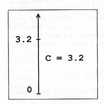
When applying real numbers full machinery of numerical mathematics can be applied. Among other things implicit ordering of the values is provided. But a tool relying only on real numbers forces the user to model everything accurately.
One way to represent uncertainty of process parameters and process state is to use intervals of real numbers22Probability distributions are another common way to represent uncertainty. Applying them requires some knowledge or assumptions about the nature of uncertainty. Applying intervals gives as a result what is possible and what is impossible while applying probability distributions gives as a result a distribution telling how probable different values are., Fig. 3.
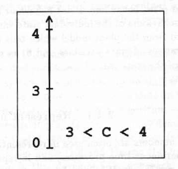
Using intervals in addition to real numbers makes it possible to express more of the available knowledge. Discrete-event control strategies rely on interval-based information on plant state. Safety margins of plant operation are often given as intervals. On intervals of real numbers the conventional mathematical operations and algorithms can be applied.
Numeric intervals carry implicit information on the ordering of the limit values. When using numeric values and computations based on them, a lot of implicit knowledge is used. This may have implications difficult to realize. Thus, when numeric values are used, they should reflect the actual system. If the user is forced to use numeric intervals when no quantitative information actually is available, he has to ‘invent’ numeric values for the parameters. At this process some invalid knowledge may easily be introduced because of the implicit mathematic relations of numeric values, especially the ordering. For such systems it is necessary to provide the user purely qualitative methods, Fig. 4.
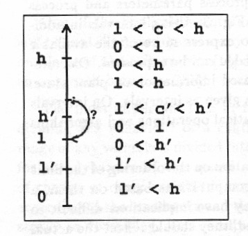
Notice that the inequalities in the figure do not tell if . To achieve something similar in quantitative problem solving we must define for example that .
Higher level reasoning in early design and diagnosis often relies strongly on symbolic values and on ordinal relations between them. The QSIM algorithm is based on this kind of knowledge. It has an algorithm of its own to handle relations like add(X,Y,Z) and mult(X,Y,Z) between symbolic intervals. The modeller can choose to which extent the ordinal relations of the landmarks of the variables are given. Another difference to using real intervals is that there is no measure of difference, only ordinal relations. This allows flexible representation of abstract incomplete knowledge so that all the knowledge is explicitly presented.
There are also symbolic values which have no ordering, Fig. 5. Various relations between them can be specified explicitly using logic clauses.
2.4.2 Representing dynamic behaviour
System behaviour can be represented as a combination of the behaviours of the state variables. The behaviour of a real-valued signal is a trend curve which tells the value of the signal at every time point, Fig. 6.
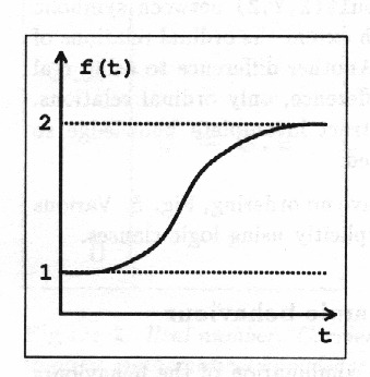
Such a trend curve is a useful piece of information for a human expert but it is difficult to use as such in further automatic analysis. The more so because to reflect uncertainty a set of trend curves is needed.
With interval representation the trend curve can be divided into episodes during which the curve experiences no qualitatively significant change, i.e. no change in the sign of the first (and the second) derivative; Fig. 7.
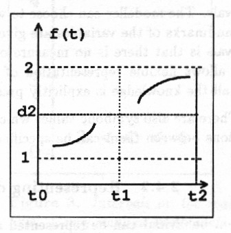
Each episode is specified using upper and lower limits, start and end time of the episode and the shape of the curve determined by the sign of the first (and the second) derivative. All or some of the limits are given as symbolic values only. Start and end points of an episode can be given either as real numbers or as intervals of real numbers or as symbolic values.
The origianl QSIM-algorithm directly generates such a qualitative representation of the behaviour using symbolic knowledge only as in Fig. 8.
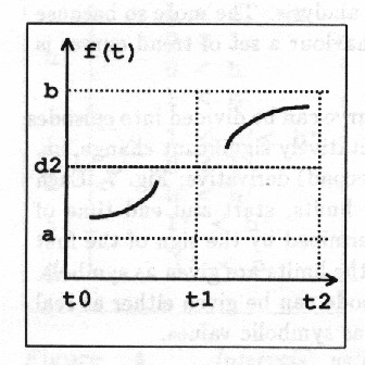
Later modifications of QSIM allow the use of quantitative knowledge when it is available to refine the prediction.
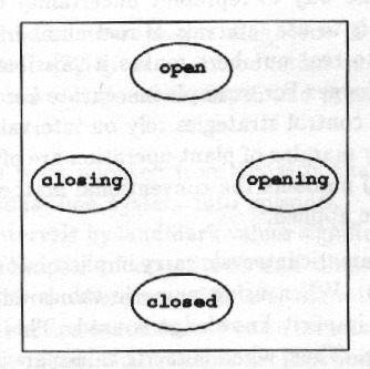
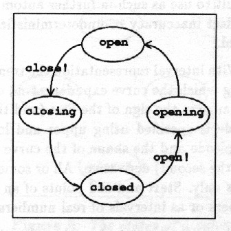
A state automaton is a natural representation of the behaviour of a system whose states are represented using symbolic discrete values, Fig. 9.
The trend curve of Fig. 6 is less appropriate for many purposes, for example for the design of discrete-event control, than the episodes in Fig. 7. The trend curve must be represented as a long sequence of real numbers while the episode representation requires only two records carrying the initial and final value of the episodes and the signs of the derivatives. It is also important to notice that the episode representation is uniform with the representation in Fig. 9. This aspect is demonstrated further below.
2.4.3 Behaviour of a simple dynamic system
Fig. 10 shows how a phase-portrait of a continuous-time dynamic system can be transformed into a state-automaton which gives a general description of the system behaviour. Such a state automaton can directly be made use of in automated reasoning.
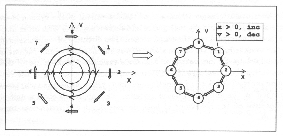
The state space is discretized according to the landmark values which are significant for the dynamics or for the outside observer. In this case the only significant landmarks are and because on those lines and change sign.
The direction of change is discretized to three values, increasing,
decreasing and steady. The signs of the derivatives in each region (= discrete state) determine the possible transitions between states. As a result the time gets divided into intervals separated by distinguished time points at which the system experiences some qualitatively significant changes. No attention is paid on knowing accurately the trajectories but the values of the state variables are rather given as relations to significant threshold values together with the direction of change. Even such a rough view on plant behaviour is sufficient for designing discrete control actions to control the plant.
From such a model the upper and lower limits of the durations of the time intervals can sometimes be approximated but exact durations can seldom be determined. However, more important than to know the time exactly is to know the order in which the significant events occur. When there is a lot of concurrent behaviour, even exact information on timing does not tell that order, because the initiating events of many phenomena are typically asynchronous.
Summary
The lines or surfaces on which any of the derivatives of the system state variables vanish divide the state space into regions together with other lines marking some significant threshold values. The direction of the movement of the system inside the regions and across the borders of the regions is determined by the derivatives of the state variables. Making use of this observation the knowledge in the system equations can be used in the reasoning on the behaviour of a continuous time system using the techniques provided by the knowledge-based systems. This approach gives a unified perspective on the behaviour of both discrete-event and continuous-time systems.
[14] presents a living example — KSE system monitoring nuclear power plant power supplies — on model-based reasoning. The paper also introduces the concepts of ‘deep knowledge’ and ‘shallow knowledge’ and discusses the benefits of applying mode-based reasoning rather than first-generation expert systems. Evolution prospects of the same approach on other plant systems is discussed as well as objectives of such evolution.
3 CONSTRAINT LOGIC PROGRAMMING
Because discrete phenomena are so important in plant control, it is natural to consider logic programming as a tool to implement algorithms to support control system design and plant operation. However, many plant properties are most naturally represented with mathematical equations, not with logic clauses, and the main phenomena taking place in a plant have continuous time dynamics. The ISIR-algorithm addresses especially the problem of dealing with systems having both discrete and continuous dynamics and which are modelled partially with mathematical equations, partially with logic clauses.
Constraint logic programming languages have special features which make them especially suitable for handling this kind of problems. A constraint logic program is a set of mathematical equations and axioms of first order logic. The inference engine determines if the set of constraints is satisfiable and if so, which subregion of the parameter space satisfies the constraints.
In this section constraint logic programming is demonstrated with various examples and its use in solving some basic algorithmic problems of the ISIR program is also explained. This is done by the following steps:
- Programming language:
-
A brief introduction of the semantics of logic programming, constraint logic programming and CLP() is given.
- Verification:
-
An essential part of the implementation of ISIR has a special structure. Some general rules on ‘informal verification’ of programs with such a structure are given.
- Discrete dynamics:
-
The ISIR-algorithm is based on considering the system behaviour as a directed graph called reachability graph or state graph. The concept of reachability graph is introduced and an example on reachability graph generation is given.
- Using constraints:
-
An example on applying pure CLP() on a ‘routing’ problem described with linear equations only is presented. Solving nonlinear equations is discussed.
- ‘freeze’:
-
A technique to reduce the complexity of the computation is presented.
- Intervals:
-
The ISIR-algorithm represents quantitative knowledge as intervals of real numbers. The principle of the interval computation utilised in ISIR is explained and demonstrated. The approach is based on global optimisation contrary to many other approaches utilizing specific interval operators and local propagation.
3.1 SEMANTICS OF THE LANGUAGE
In this and the later sections programming language CLP() is used as a representation language. For those familiar with Prolog reading CLP() programs should be easy. The main difference is that the operator is is not defined and -sign should be used instead. Consequently a clause X = Y + Z is not a rule how to compute X but a relation which X and Y must satisfy. Because CLP() interpreter can solve mathematical equations in addition to logic problems CLP() can be seen as an extension of Prolog on the domain of real numbers.
The execution order of the program is not strictly from left to right as in Prolog because of the need to handle properly the mathematical constraints. For example the CLP() interpreter delays the equation X = Y + Z until there is enough information to solve X,Y Z, i.e. more equations with X,Y and Z are encountered or some of the values of X,Y and Z are given in the program.
A Prolog program is a collection of facts about objects [7]. likes(john, beer) tells about objects john and beer the fact that the relation ‘john likes beer’ stands between them. A variable can be used to stand for any object in a relation. Any name beginning with a capital letter is taken to be a variable. The names of the relations, for example likes above, cannot be variables.
The following examples from [27] illustrate the semantics of Prolog. The Prolog program
sister(X,Y):-
    dif(X,Y),parent(X,Person), parent(Y,Person).
can be transformed into the predicate logic clause
and further into
Which can be read as “for all and stands that they are sisters if there exists somebody who is the parent for both of them and if and are different”.
The program
parent(X,Y):- mother(X,Y).
parent(X,Y):- father(X,Y).
can be written in predicate logic as
which can be read as “for all and it stands that is a parent of if is the mother of or if is the father of ”.
The facts on family relations can be presented as follows:
mother(maija,eeva).
mother(kaisa,eeva).
mother(annastiina,maija).
mother(ilona,maija).
father(kaisa,risto).
The program is executed by making a query, which is simply a relation which may have some variables in it. The Prolog interpreter checks if the relation is in accordance with facts and relations given in the program, i.e. if the relation in the query can be deduced from the facts and the relations in the program. In doing this the interpreter ‘fills in’ appropriate values for the variables as shown below:
SICStus 0.6 #18: Fri Jun 11 11:18:28 CDT 1993
Copyright (C) 1987, Swedish Institute of Computer Science.
All rights reserved.

| ?- sister(maija,X).
X = kaisa
yes
maija has a sister whose name is kaisa.
If there are alternative solutions they can be found by rejecting the first solution.
| ?- mother(maija,risto).
no

| ?- mother(maija,X).
X = eeva ? ;
no

| ?- mother(X,eeva).
X = maija ? ;
X = kaisa ? ;
no

| ?- father(X,Y).
X = kaisa, Y = risto ? ;
no
Prolog applies so called ‘closed world assumption’ which means that a fact not explicitly stated in the program is false. For example, according to the above program jane has neither father nor mother because there is not a corresponding relation in the program.
Constraint logic programs have in principle the same semantics as ordinary Prolog programs but the constraint approach requires different implementation of the language and it allows more efficient programming techniques. The predicate dif(X,Y) in the above program is actually a constraint — it constrains the possible values of X and Y. In standard Prolog the test on inequality of two uninstantiated variables is meaningless so that a corresponding test should be made only after it is certain the variables are instantiated.
Standard Prolog has no built-in capability to solve mathematical problems. CLP() is a constraint logic programming language which can solve linear equations and inequalities and to some extent also nonlinear equations. In effect this means that the relations in the program can be mathematical equations and inequalities in addition to logic clauses.
CLP(R) Version 1.2
(c) Copyright International Business Machines Corporation
1989 (1991, 1992) All Rights Reserved

eq(X,Y,Z):-                             3 ?- eq(X,-2,Z).
   X > 0,                               Z = 4
   X + Y = Z,                           X = 6
   X - Y = 2*Z.                         *** Yes

1 ?- eq(X,Y,Z).                         4 ?- eq(X,Y,1).
Y = -0.5*Z                              Y = -0.5
X = 1.5*Z                               X = 1.5
0 < Z                                   *** Yes
*** Yes

2 ?- eq(1,Y,Z).
Z = 0.666667
Y = -0.333333
*** Yes
In appendix A Prolog and CLP() are presented in more detail and with more examples.
3.2 SOME CORRECTNESS CHECKS OF CONSTRAINT LOGIC PROGRAMS
There is no way to prove the absolute correctness of programs, but explicit consideration of certain topics increases the confidence on the programs.
Much of the ISIR-algorithm is implemented applying a common constrain-and-generate (often called test-and-generate) programming technique. In this approach there is a generator spanning the whole problem space by producing all the possible combinations of the allowed values of the variables. From this space non-solutions are excluded with various constraints. Dividing the problem solution into two — generation of all the alternatives in the problem space, and testing which of the alternatives are solutions — makes the programming much easier to compare to programming an explicit solution. In addition test-and-generate solutions are more flexible than programs applying fixed procedural algorithms: they can solve a wider range of problems and they are easier to modify to solve new types of problems.
The above benefits are achieved with the expense of computation time. To avoid going through the whole search base the constraints are ‘executed’ first as in the example in Table 1 which searches for all the combinations of three integers in a given set whose sum is in a given range:
test_and_generate:-
   set_counter(iter,0),
   test(X,Y,Z,Sum),
   generate(X),
   generate(Y),
   generate(Z),
   add_counter(iter,1),
   printf(
    'x: %  y: %  z: %  sum: %\n',
     [X,Y,Z,Sum]),
   fail.
test_and_generate:-
   counter_value(iter,Trials),
   printf('% trials',[Trials]).

test(X,Y,Z,Sum):-
   X+Y+Z = Sum,
   2 <= Sum, Sum <= 3.
generate(-2). generate(-1).
generate(1). generate(2).
generate(3). generate(4).

1 ?- test_and_generate.
x: -2  y: 1  z: 3  sum: 2
x: -2  y: 1  z: 4  sum: 3
x: -2  y: 2  z: 2  sum: 2
  .
     .
        .
x: 3  y: 1  z: -1  sum: 3
x: 3  y: 2  z: -2  sum: 3
x: 4  y: -2  z: 1  sum: 3
x: 4  y: -1  z: -1  sum: 2
x: 4  y: 1  z: -2  sum: 3
40 trials
*** Yes
In the example the test tells which alternatives are acceptable. It is also possible to construct tests telling which alternatives are unacceptable and that all the alternatives which are not explicitly stated as unacceptable are acceptable. Note that only 40 alternatives are fully generated although there are altogether alternatives.
The following checks should be made on constrain-and-generate programs.
-
1.
Check that the generator base contains all the actual solutions.
The solutions are searched only among the alternatives provided by the generator. In most cases constructing and verifying the generator is straightforward.
-
2.
Check that the constraints do not exclude any solutions.
The tests usually consist of many separate constraints which can be verified one by one making the verification simple. However, there is one pitfall when using languages like CLP() which apply the closed world assumption: All the alternatives not considered in the test are excluded because the test fails. When the test is composed of many individual predicates it is not easy to see which part of the generator space is actually covered. Thus, during the verification it is a good idea to check for which range of the generator space the tests are defined.
In some special cases the goal may be to find one solution. Then it is sufficient that not all the solutions are excluded.
-
3.
Check that the constraints exclude all the non-solutions.
The constraints must be constructed to have an easy to understand structure to avoid any non-solutions to be accepted. Automatic checking on which alternatives the individual tests succeed and fail can reveal errors.
If the goal is to check that nothing can ever go wrong, then not succeeding to exclude all the non-solutions only poses some extra safety requirements for the system under analysis.
-
4.
Check that the computation will end.
Error in the program structure (typically in the end condition of recursion) or an uninstantiated end condition of recursion may cause infinite computation. The former error will be revealed in the first test and thus causes troubles to the program developer only. But the latter may pass the tests unnoticed causing the user troubles whose reason is difficult to identify.
-
5.
Explain the reason for using assert, retract, cut, if-then-else structures and other non-logical features.
Meta-logical features are easily used more often than necessary in logic programming. Because they break the clear logic structure of the programs special discipline must be obeyed when they are used.
-
6.
If dynamic predicates are used, check that they are properly initialised.
Assert and retract cause meta-logical side-effects whose effect may persist even from one execution of program to the execution of another program if appropriate initializations are not made.
-
7.
List the special assumptions on e.g. initial instantiation of the variables.
Use of meta-logical features may limit the applicability of the program for example by requiring that some of the arguments in the top-level predicate must be initially instantiated. Such limitations must be made explicit in the documentation or preferably additional test on correct initialisation should be included in the program.
The above can be applied in a hierarchic manner on the program modules.
3.3 REACHABILITY GRAPH OF A DISCRETE-EVENT SYSTEM
A discrete-event system experiences discrete state transitions ( events) which take the system from one discrete state to another. Thus, the behaviour of a discrete-event system can be represented as a directed graph called a reachability graph because it tells which states can be reached from an initial state. The analysis of the dynamics of discrete-event systems is commonly based on the reachability graph.
The reachability graph is generated using axioms telling the relationships of the system variables and the changes which they may experience. To demonstrate how the reachability graph is generated, a childrens’ game is studied as an example of a typical discrete-event control problem.
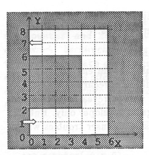
In the game an object is moved in steps on a track like for example the one in Fig. 11. The object has a velocity in the x- and the y-direction. The velocity can be increased or decreased with one unit in each step. At each step the object is moved as many units of distance as the velocity indicates. The goal is to reach the end of the track with as few steps as possible.
Moving the object according to the rules, marking every position of the object and drawing an arrow from one position to the next one gives a state graph33Actually it is not sufficient to consider the position of the object as its state but its velocity must also be considered.. Trying out all the alternatives gives a state graph which represents all the legal possible paths from start to goal in a compact way. The following example shows how such a graph can be generated automatically.
For the purposes of the analysis the track is defined in CLP() as a predicate track(S) in Table 2, which is true if the object is on the track and it is moving in the allowed direction. The rules of movement can be given as in Table 3.
track(S)
- S:
the state of the object represented as a structure st(X,Y,Vx,Vy)
- X, Y:
the x- and y-positions of the object
- Vx, Vy:
velocities in x- and y-directions.
track(st(X,Y,Vx,_)):-
         0 <= X, X < 4, 0 <= Y, Y <= 2, Vx > 0.
track(st(X,Y,Vx,Vy)):-
         4 <= X, X <= 6, 0 <= Y, Y <= 2, Vx > 0, Vy > 0.
track(st(X,Y,_,Vy)):-
         4 <= X, X <= 6, 2 < Y, Y < 6, Vy > 0.
track(st(X,Y,Vx,Vy)):-
         4 <= X, X <= 6, 6 <= Y, Y <= 8, Vx < 0,Vy > 0.
track(st(X,Y,Vx,_)):-
         0 <= X, X < 4, 6 <= Y, Y <= 8, Vx <= 0.
step(S0,S)
- S0:
state before the move
- S:
state after the move.
step(st(X0,Y0,Vx0,Vy0),st(X0+Vx,Y0+Vy,Vx,Vy)):-
       speed(Vx0,Vx), speed(Vy0,Vy).

speed(V0,V0+1).  speed(V0,V0-1).  speed(V0,V0).
The reachability graph of an object moving on the track can now be generated by calling the predicate path(0,st(0,1,0,0)) where st(0,1,0,0) is the initial state representing the position (0,1) and zero velocity; see Table 4.
path(M,S0,Len0,Max)
- M:
Id. number of the current state
- S0:
current state
- Len0:
the number of steps taken this far
- Max:
maximum allowed number of steps
path(M,S0,Len0,Max):-
      Len0 < Max,
      step(S0,S),               % step further
      not(S0 = S),              % really moving on ?
      track(S),                 % on the track ?
      is_new(M,N,S),            % not been here before ?
      Len = Len0 + 1,
      path(N,S,Len,Max).        % proceed
The first argument M is the identification number of the current state and the second argument S0 is the current state. Recursion on this branch is finished if the maximum number of steps is exceeded ( Len0 Max). A new possible state is generated using the rules of moving the object one step ( step(S0,S)). Because the rules do not forbid stopping it is checked that the result is a state different from the current one ( not(S0 S)). According to the rules the new position must be on the track ( track(S)). Because all the paths will be passed and because separate paths may join, it is necessary to check that the state S really is a ‘new’ one, not one belonging to a path which has already been passed ( is_new(M,N,S)). If all the above conditions are true, then the algorithm proceeds along the path ( path(N,S,Len,Max)). If any one of the above conditions fails, then the algorithm backtracks and tries other alternatives, if any. (In effect it retries step(S0,S).) 44The algorithm presented here is not the only possibility. Another common alternative to solve this kind of problems avoids the use of assert by storing the graph in a list instead.
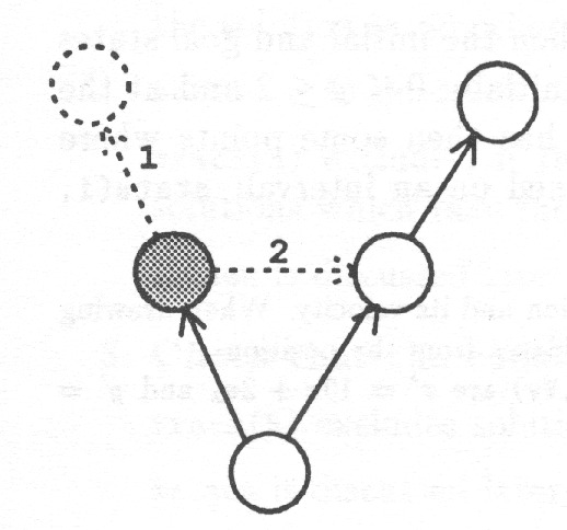
All the states and transitions passed must be stored for later comparison with new states and transitions. The predicate is_new in Table 5 compares the state with those already generated and stores it if it is a new state (see Fig. 12);
is_new(M,N,S)
- M:
id number of the current state
- N:
id. number of the next state
- S:
new state to be checked
is_new(M,_,S):-
     state(K,S),          % not a new state
     not(trans(M,K)),     % but a new way to get there
     assert(trans(M,K)),  % insert the transition
     fail.                % but do not proceed in this direction

is_new(M,N,S):-
     not(state(_,S)),     % a new state
     get_number(N),       % give it a unique name
     assert(state(N,S)),  % insert the state
     assert(trans(M,N)),  % and the transition
     printf('new state % % -> %\n',[S,M,N]).
-
•
If there is already a similar state ( state(K,S)) but there is not a transition from the current state to it ( not(trans(M,K))), then a new transition has been detected and a corresponding edge will be inserted into the graph ( assert(trans(M,K)). However, there is no need to proceed in this direction ( fail).
-
•
There is not yet a similar state ( not(state(_,S))) in a graph, and both the state and the transition to it must be inserted ( assert(state(N,S)), assert(trans(M,N))). In this case the graph generation must proceed in this direction.
-
•
If there is already a similar state and a transition from the current state to that state in the state graph (both the definitions of is_new fails), then nothing new to insert in the graph has been found.
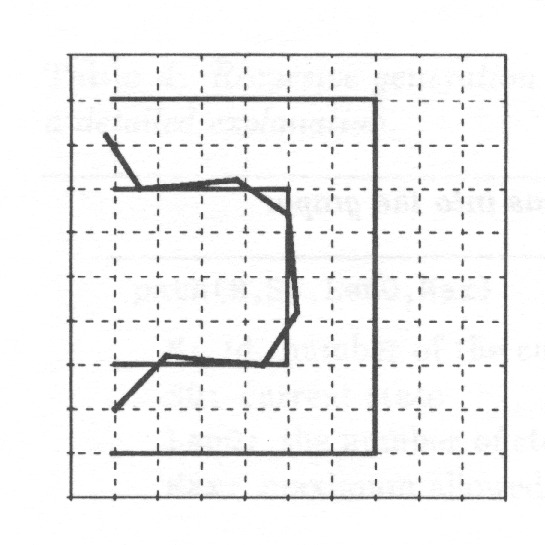
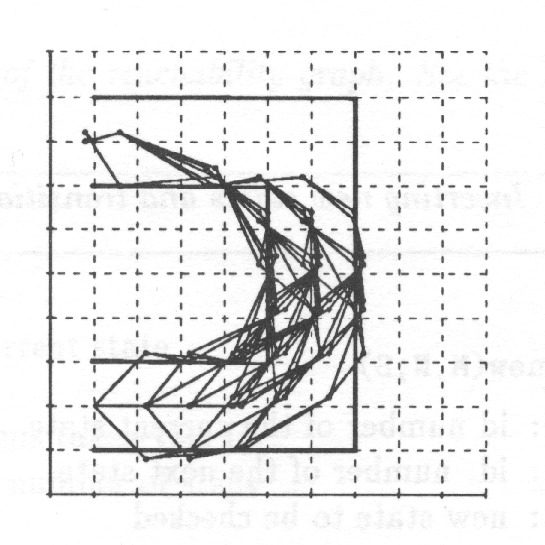
Fig. 13 shows one path of the state graph taking the object from the initial state to the final one.
Fig. 14 shows all the paths which take the object into the final state in 8 steps.
It is possible to solve the problem even when the initial and goal states are only partially defined by requiring that initially and at the goal state . The resulting track has then some points where y does not have a real value but is constrained on an interval: state(1, st(1, _1, 1, 1)):- _1 <= 2, - _1 <= -1.
3.3.1 Summary
A generally applicable predicate path is presented for the analysis of discrete systems for which and where the additional constraints are of the form where is a set of equations and inequalities. Naturally and can also contain logic clauses. An approach similar to the one in the above example is applied in the ISIR-algorithm.
3.3.2 Correctness proof of the reachability graph generation
The predicates path and is_new in the previous section are evaluated according to the principles presented in section 3.2.
Checking the predicate path
-
1.
Check that the generator base contains all the actual solutions.
step(S0,S) gives, if the track is correctly specified, a successor for the state S0. On backtracking it gives another alternative successor or fails if there are no more alternative successors.
If neither track(S) nor is_new(M,N,S) fails at least path(N, S, Len, Max) will fail; if not earlier at least when the condition Len0 < Max becomes false. Thus the program will finally always backtrack and all the alternatives provided by step(S0,S) will be tried. Because path is recursive, the above applies also to all the successors of S0.
-
2.
Check that the constraints do not exclude any solutions.
len0 < Max limits the maximum depth of the search but constrains the solution in no other way.
not(S0 = S) does not exclude any solutions.
track(S) excludes, if the system is correctly specified, only illegal solutions which take the object outside the track.
is_new is discussed later.
-
3.
Check that the constraints exclude all the non-solutions.
track(S) excludes solutions which take the object outside the track.
is_new is discussed later.
-
4.
Check that the computation will end.
The predicate path has only one definition. In each step forward the parameter Len is increased by one. Thus the recursion is limited by the condition Len0 < Max.
-
5.
Explain the reason for using assert, retract, cut, if-then-else structures and other non-logical features
None used.
-
6.
If dynamic predicates are used, check that they are properly initialised.
None used.
-
7.
List the special assumptions on e.g. initial instantiation of the variables.
It is not necessary to define completely either the initial or the final state, but the instantiations should define a solvable problem to guarantee that the computation will end.
The id. number of either the initial or the goal should be instantiated to get the id. numbers for the states.
Checking the predicate is_new
-
1.
Check that the generator base contains all the actual solutions.
Because is_new is used purely as a constraint this is not relevant.
-
2.
Check that the constraints do not exclude any solutions.
is_new prevents ‘looping’. It inhibits recursion from states already analyzed. The first rule fails when the state S generated by step(S0,S) is already in the graph. Proceeding with the recursion from such a state would give no new solutions. The second rule succeeds when S is a new state.
-
3.
Check that the constraints exclude all the non-solutions.
Non-solutions will not appear as an argument of is_new. Its task is to store the graph and avoid infinite looping in the computation.
-
4.
Check that the computation will end.
is_new inserts state S into the graph if it does not already exist there. It also inserts the edge S0 S if it is not yet inserted. Insertion is accomplished by assert and there is no retract in the algorithm.
is_new prevents the recursion from passing twice through the same edge in the graph. Thus, if the graph has a finite number of edges the computation will end.
-
5.
Explain the reason for using assert, retract, cut, if-then-else structures and other non-logical features.
Assert is used only to incrementally build the state graph.
-
6.
If dynamic predicates are used, check that they are properly initialised.
In the examples the following instantiations are used:
         retractall(state(_,_)),
         assert(state(0,st(0,1,0,0))),
         retractall(trans(_,_)),
         setcounter(counter,0),
Hence all the dynamic variables are properly initialised.
-
7.
List the special assumptions on e.g. initial instantiation of the variables.
There are no special assumptions. To get an instantiated solution it is necessary to have the problem sufficiently well defined.
3.4 APPLYING CONSTRAINT EQUATIONS
The ISIR-algorithm is based on the CLP() programming language which is a generalisation of the programming language Prolog. CLP() allows also the use of mathematical equations and inequalities in programs. The following exemplifies what can be achieved with pure CLP().
3.4.1 Structural reasoning
Finding a route to transfer material from one place to another in a large network of pipes, valves and pumps is a typical problem in the operation of process plants. Sometimes it is necessary, in addition to finding a route, also to take into account some quantitative constraints or to satisfy some quantitative requirements.
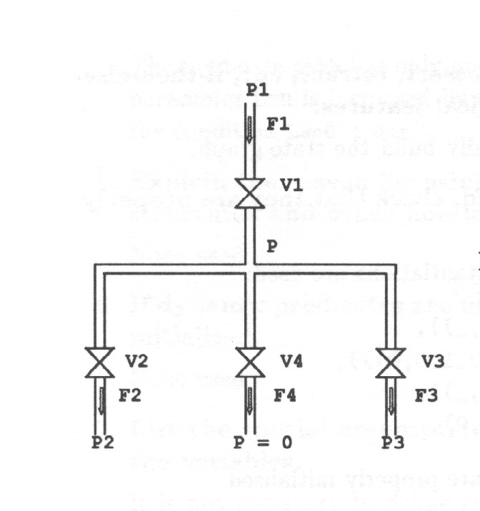
The system in Fig. 15 is given a specification in Table 6 to demonstrate how to solve such routing problems.
net(P1,P2,P3,P,F1,F2,F3,F4,V1,V2,V3,V4):-
      valve(V1, P1 - P, F1, G1),
      valve(V2, P - P2, F2, G2),
      valve(V3, P - P3, F3, G3),
      valve(V4, P, F4, G4),
      F1 = F2 + F3 + F4,
      valve_params(G1,G2,G3,G4).

valve(open,Dp,F,G):- F = G*Dp.
valve(closed,_,0,_).

valve_params(0.1,0.3,0.6,1).
where
valve(State,Pressure,Flow,Flow_coeff)
- State:
the state of the valve, open or closed
- Pressure:
pressure difference over the valve
- Flow:
flow through the valve
- Flow_coeff:
‘conductance’ of the valve
The flow through the valve is modelled to be proportional to the pressure difference when the valve is open. When the valve is closed the flow is modelled to be zero and the pressure is left free. The four valves in the system are required to satisfy the relation defined by the valve model and the pressures and flows are required to be those given in 15. In addition it is stated that there is no conservation of mass.
The model can be used to solve for example under which conditions or when the pressures are known. As the results in Table 7 show making is impossible.
?- net(P1, P2, P3, P, F1, F2, F3, F4, V1, V2, V3, V4),
       P1 = 10, P2 = 6, P3 = 3, F4 > 1, F4 < 2.
| V4 open | V3 open | V2 closed | V1 open |
| F4 1.64706 | F3 -0.811765 | F2 0 | F1 0.835294 |
| P 1.64706 | P3 3 | P2 6 | P1 10 |
| V4 open | V3 open | V2 open | V1 closed |
| F4 1.89474 | F3 -0.663158 | F2 -1.23158 | F1 0 |
| P 1.89474 | P3 3 | P2 6 | P1 10 |
| V4 open | V3 closed | V2 open | V1 closed |
| F4 1.38462 | F3 0 | F2 -1.38462 | F1 0 |
| P 1.38462 | P3 3 | P2 6 | P1 10 |
| V4 open | V3 open | V2 closed | V1 closed |
| F4 1.125 | F3 -1.125 | F2 0 | F1 0 |
| P 1.125 | P3 3 | P2 6 | P1 10 |
?- net(P1, P2, P3, P, F1, F2, F3, F4, V1, V2, V3, V4),
       P1 = 10, P2 = 6, P3 = 3, F4 > 3.
*** No
The above approach may be of practical use, but often the uncertainty of the parameters should be taken into account. Because pressures and characteristics of the valves are seldom known exactly, relying on a single value will give misleading results. For example in some cases the actual flow may have a direction opposite to the one predicted by the model only because of a small error in the model parameters. This is especially important when there are nonlinearities in the models. In the approach taken in this report the values of the variables are intervals rather than single point values. Determining regions of possible solutions rather than single point values results in implicit sensitivity analysis.
There is also another point of view on uncertainty: Because many problems can be solved without exactly knowing the parameters the problem solving tools should not require the extra trouble of finding out the exact values of the parameters.
It is not always easy to see when a problem is under- and when over-determined. If the flow had been exactly determined there would have been no solution. Had one of the valve coefficients been undefined, there would have been no solution. It is much easier to use a tool which always gives some solution that helps in reformulating the problem than a tool which gives a solution only after the problem is formulated well enough. The interval approach taken here assumes the initial value for any variable not assigned explicitly a value. Thus there is always a solution which can then be further adjusted by constraints excluding unreasonable values.
3.4.2 Solving systems of nonlinear equations
CLP() can solve any set of linear equations and inequalities (in addition to Prolog-like logic constraints). It can also deal with non-linear constraints to some extent by ‘putting them aside’ to wait for some of the variables in them to get solved so that the constraint becomes linear. For example is a nonlinear constraint but after executing constraints it becomes linear because gets solved.
In terms of the procedural semantics of Prolog, non-linear CLP() constraints always succeed in allowing the execution to continue and not forcing the program to backtrack. Backtracking occurs only later if it turns out, due to some of the variables getting instantiated, that the non-linear constraint cannot be satisfied. In the previous example on the valves, the constraints of the form are handled properly, because in course of the execution either x or y is instantiated thus making the constraint linear.
If there is a constraint then can be solved when is instantiated (i.e. known) but not vice versa. But if a constraint is added in the program, then also can be solved when is known. If the set of constraints contains an (implicit) second order equation, the solution formula of the second order equation can be added into the constraints so that CLP() can solve them. The predicate polynom(X,Y) in Table 8 implements a solution to the equation .
polynom(X,Y):- sec_ord(1,-3,2-Y,X).

% imaginary roots omitted
sec_ord(A,B,C,X):-
     A*X*X + B*X + C = 0,
     Tmp = pow(B*B - 4*A*C,0.5),
     sec_ord2(A,B,Tmp,X).

sec_ord2(A,B,Tmp,X):- Tmp > 0, 2*A*X = -B + Tmp.
sec_ord2(A,B,Tmp,X):- Tmp > 0, 2*A*X = -B - Tmp.
sec_ord2(A,-2*A*X,Tmp,X).
In Table 9, or is solved using polynom(X,Y).
1 ?- polynom(1,Y).
Y = 0
*** Yes

2 ?- polynom(0,Y).
Y = 2
*** Yes

3 ?- polynom(X,1).
X = 2.61803
*** Retry? y
X = 0.381966
*** Yes
4 ?- polynom(X,Y).
2*X - 3 = pow(4*Y + 1, 0.5)
Y + 3*X - 2 = X * X
Y + 3*X - 2 = X * X
*** Retry? y
-2*X + 3 = pow(4*Y + 1, 0.5)
Y + 3*X - 2 = X * X
Y + 3*X - 2 = X * X
*** Maybe
The more there are nonlinear equations, the more the above approach resembles a sort of local propagation, in which the equations are like separate constraints through which the known values of the variables are propagated. When implemented in CLP() it is more than pure local propagation because the constraints become linear after some variable assignments are solved globally, but still it is not guaranteed that all the problems which have analytic solutions can be solved with this approach. To always find the solutions, the whole set of constraints must be analyzed and all the non-linearities which are ‘coupled’ together must be given an explicit analytic solution as a simultaneous set of non-linear equations.
3.5 FREEZING UNINSTANTIATED CONSTRAINTS
Internally CLP() delays non-linear constraints until they become linear when some of the variables involved get solved. The same approach can be applied as well on other cases to reduce the complexity of the computation.
dem_frz0:-
  set_counter(n,0),
  y(B),
  polynom(A,B),
  polynom(C,D),
  add_counter(n,1),
  A < 0.2, C < 1,
  y(D),
  printf('a:% b:% c:% d:%\n',
  [A,B,C,D]),
  fail.
dem_frz0:-
  counter_value(n,N),
  printf('% trials',[N]).
y(0).  y(1).  y(2).

3 ?- dem_frz0.
a: 0  b: 2  c: 0.382  d: 1
a: 0  b: 2  c: 0  d: 2
18 trials
*** Yes
The piece of code in Table 10 solves two second order equations for values under given additional requirements on the solutions. Increasing the counter ‘n’ ( add_counter(n,1)) is meant to represent some complex computation.
dem_frz1:-
  set_counter(n,0),
  y(B),
  polynom(A,B,Frz1),
  polynom(C,D,Frz2),
  add_counter(n,1),
  A < 0.2, C < 1,
  y(D),
  freezed([Frz1,Frz2],[]),
  printf('a: % b: % c: %
     d: %\n', [A,B,C,D]),
  fail.
dem_frz1:-
  counter_value(n,N),
  printf('% trials',[N]).
polynom(X,Y,Frz):-
   Y = X*X - 3*X + 2,
   sec_ord(1,-3,2-Y,X,Frz).

% imaginary roots omitted
sec_ord(A,B,C,X,Frz):-
   A*X*X + B*X + C = 0,
   Tmp = pow(B*B - 4*A*C,0.5),
   Frz = freeze(Tmp,
         sec_ord2(A,B,Tmp,X)).

4 ?- dem_frz1.
a: 0  b: 2  c: 0.381966  d: 1
a: 0  b: 2  c: 0  d: 2
3 trials
*** Yes
The output in Table 10 shows that there are two solutions and that the counter is passed 18 times. Most of the calls to sec_ord are unnecessary because they occur during backtracking when A 0.2 fails. In such cases trying out the other solution is unnecessary because the condition will fail until B gets another value.
In the example in Table 11 calling the predicate sec_ord2 is postponed until all the variables needed in obtaining a solution are instantiated. Thus a ground result is obtained and it can be directly used further in the constraints. Inconsistent results are noticed immediately and much less computation is needed.
Freezing, i.e. postponing or delaying the call of sec_ord2 is accomplished by gathering calls to it in a list and processing them later by calling the freezed-predicate. The same result as before is obtained but this time the counter is passed only 3 times.
The above example was artificially constructed to demonstrate the effect of freezing some constraints. In the example the complexity could have been reduced by reorganising the code, but in general such reorganising is very difficult especially in large programs. The more so because the optimal order of the constraints depends on the order in which the variables get instantiated, which cannot be assumed to be known when constructing programs for general problem solving.
Because CLP() does not currently have means to freeze goals selected by the user, freezing is implemented using the predicates in Table 1266There are Prolog dialects which provide ‘freeze’ as an internally implemented feature. Maybe it, or something more general, will be implemented in CLP() as well..
The alternatives of frozen correspond to the following cases:
-
1.
All the delayed goals are executed.
-
2.
No more delayed goals can be executed before some more variables get instantiated. Some frozen goals remained as a residue.
-
3.
One run through the list of frozen goals is finished. Start a new run to check if the goals executed during the previous run made possible to execute still some more.
-
4.
Process one frozen goal. The lock is ground and the goal can be executed.
-
5.
Process one frozen goal. Because the lock is not ground, the goal cannot be executed.
freezed(Frozen, Residue)
-
Frozen:
Delayed goals,
-
Residue:
Goals which could not yet be executed.
frozen(Frozen, Unprocessed, Switch, Residue)
-
Frozen:
Delayed goals
-
Unprocessed:
Collection of goals which could not be executed yet.
-
Switch:
tells if any of the goals has been executed. Used to control the repeated processing of the list of frozen goals.
-
Residue:
Goals which could not be executed yet.
freezed(Frozen,Residue):- frozen(Frozen,[],f,Residue).

frozen([],[],t,[]):- !.                                    % 1
frozen([],Frozen,f,Frozen):- !.                            % 2
frozen([],Frozen,t,Residue):- frozen(Frozen,[],f,Residue). % 3
frozen([freeze(Lock,Goal)|T],Frozen,_,Residue):-           % 4
      ground(Lock),
      call(Goal),
      frozen(T,Frozen,t,Residue).
frozen([freeze(Lock,Goal)|T],Frozen,Switch,Residue):-      % 5
      nonground(Lock),
      frozen(T,[freeze(Lock,Goal)|Frozen],Switch,Residue).
In the above examples the benefits of freezing were demonstrated by counting the times a part of the code is executed. It has been tested that freezing implemented even with the above inefficient metalevel approach can reduce also execution times drastically, and that it never increases the execution time significantly.
3.6 SOLVING INTERVAL CONSTRAINT PROBLEMS
For various reasons interval constraint problems are often encountered. For example uncertainty on a parameter c can be expressed as and plant automatics are based on discrete control actions triggered by process variables exceeding given threshold values. The previous example on the valves also showed that being able to work only on exact values is not sufficient, because of being too restrictive to require exact values of the valve parameters and pressures to be known.
The following example shows the principles of how interval constraint problems are solved in the ISIR-algorithm. Variables and are constrained into a closed region S where and . In addition they are constrained by the equations and .
In the program in Table 13 the constraint equations are first activated by calling the predicate equation(X,Y,A,B). Then every variable is assigned a value
one by one. Finally the result is printed out.
demo:-
        equation(X,Y,A,B),
        x(X), y(Y), a(A), b(B),
        dump([X,Y,A,B]),fail.

equation(X,Y,A,B):-
        X+Y = A, X*Y = B. % the constraint equation

% any variable is on the border of S or inside S
x(0).  x(10).  x(X):- 0 < X, X < 10.
y(1).  y(9).  y(Y):- 1 < Y, Y < 9.
a(-5).  a(100).  a(A):- -5 < A, A < 100.
b(2).  b(50).  b(B):- 2 < B, B < 50.
The alternative solutions are the following:
* X = 10, Y = 1, A = 11, B = 10
* X = 10, Y = 5, A = 15, B = 50
X = 10, A = Y + 10, B = 10*Y, Y < 5, 1 < Y
* X = 2, Y = 1, A = 3, B = 2
Y = 1, A = X + 1, B = X, X < 10, 2 < X
* X = 0.222222, Y = 9, A = 9.22222, B = 2,
* X = 5.55556, Y = 9, A = 14.5556, B = 50
Y = 9, A = X + 9, B = 9*X, X < 5.55556, 0.222222 < X
A = Y + X, B = 2, Y < 9, Y + X < 100, X < 10, 1 < Y
    -5 < Y + X, 0 < X, 2 = X * Y
A = Y + X, B = 50, Y < 9, Y + X < 100, X < 10, 1 < Y,
    -5 < Y + X, 0 < X, 50 = X * Y
A = Y + X, Y < 9, Y + X < 100, B < 50, X < 10, 1 < Y,
    -5 < Y + X, 0 < X, 2 < B, B = X * Y
It is evident that when the solution is a point (the results given in ground terms, marked with ‘*’ in Table 13), it represents a corner of the region S while a solution with equalities and inequalities represents a region inside S. Thus it is sufficient to pick the results given in ground terms and search the minima and maxima of the variables among them. For example it can be seen that .
The example demonstrates the test-and-generate approach. When
there is a
large set of equations it is not necessary to evaluate all of
them for all
the possible combinations. For example after
equation is called and after and have been
assigned
the values , cannot be assigned the values
or .
This is because the equation constraints are activated before
generating
values for the variables. In the example 11 solutions are fully
evaluated
while the number of all the possible combinations is .
Summary
In the above example a set of special type of optimisation problems is solved. The goals to be optimised are linear with respect to the parameters. The extremes are on the borders of the region as in linear programming. Contrary to linear programming the system equations are not necessarily linear.
3.7 CONSTRAINED OPTIMIZATION
In the previous example the minima and maxima could be found at the corners of the region. In the following example this is not the case. The equation constraint is the equation 1 and initially there is a priori knowledge that .
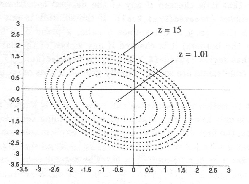
As Fig. 16 indicates it is possible to find tighter bounds for and if the equation 1 is required to be satisfied. The borders of the region and the lines where the derivatives vanish determine the potential extremes. The non-constant partial derivatives of the variables are:
| (1) | |||||
| (2) | |||||
| (3) | |||||
| (4) | |||||
| (5) |
The second-order equations must be solved explicitly. Because equation is called before any of the variables are grounded the two alternative solutions to second order equations would lead to a lot of unnecessary backtracking. Thus, solving any second order equation is postponed using the freezed-predicate until its coefficients are ground. This is done by gathering the goals into a list and, when appropriate, checking if any equation has ground coefficients.
minmax(Xlh,Ylh,Zlh):-
    equation(X,Y,Z,Frz),
    l_h(Xlh,X), l_h(Ylh,Y), l_h(Zlh,Z),
    flat(Frz,Frz1),
    freezed(Frz1,Res),
    inside(X,Y,Z),
    freezed(Res,[]),
    ground([X,Y,Z]),
    printf('x: %  y: %  z: % \n',[X,Y,Z]),
    fail.

l_h(i(L,_),L).
l_h(i(_,H),H).
l_h(i(L,H),X):- L < X, X < H.

equation(X,Y,Z,[Frz1,Frz2]):-
       3*Y*Y + 3*X*X + 2*X*Y + 4*Y + 4*X + 3 - Z = 0,
       sec_ord(3,2*X+4,3*X*X+4*X+3-Z,Y,Frz1),
       sec_ord(3,2*Y+4,3*Y*Y+4*Y+3-Z,X,Frz2).

inside(X,Y,Z):-
      Z - 1 > 0,
      Y + 3*X + 2 = 0,
      6*(2*X + 1)*(2*X + 1) =  Z - 1,
      (2*X + 1 = pow((Z - 1)/6,0.5)
       ; 2*X + 1 = -pow((Z -1)/6,0.5)).
inside(X,Y,Z):-
      Z - 1 > 0,
      3*Y + X + 2 = 0,
      6*(2*Y + 1)*(2*Y + 1) =  Z - 1,
      (2*Y + 1 = pow((Z - 1)/6,0.5)
       ; 2*Y + 1 = -pow((Z - 1)/6,0.5)).
inside(X,Y,_):- Y + 3*X + 2 = 0, 3*Y + X + 2 = 0.
inside(_,_,_):- abs(Y + 3*X + 2) > 0, abs(3*Y + X + 2) > 0.
tst:-
   Xlh = i(-3,3), Ylh = i(-2,3), Zlh = i(-5,15),
   minmax(Xlh,Ylh,Zlh).

3 ?- tst.
x:  1.63299   y: -2         z: 15
x:  -1.63299  y: -2         z: 15
x:   0        y: -2         z: 7
x:  -1.26376  y:  1.79129   z: 15
x:  -2.79129  y:  0.263763  z: 15
x:   1.79129  y: -1.26376   z: 15
x:  -0.5      y: -0.5       z: 1
Table 14 gives a solution to the problem. First the equation constraint is activated ( equation(X,Y,Z,Frz)). Then variables are constrained on the borders of the region or inside the region ( l_h(Xlh,X), l_h(Ylh,Y), l_h(Zlh,Z)). After that it is checked if any of the delayed second order equations can be solved ( freezed(Frz1,Res)). If the solution is not yet constrained enough (i.e. determines a cube, a plane or a line, not a point, inside the borders) it is checked if any zeroes of the partial derivatives lie in that region ( inside(X,Y,Z)). With freezed(Res,[]) the remaining delayed constraints are solved. Finally ground triples of are printed out.
It is important to notice that equation can solve if is known and vice versa, but if it is only known e.g. that calling equation is not sufficient. Thus, the first definition of inside gives explicit solution for the pair of equations and representing the case and . The second definition of inside represents the case and . The third alternative specifies the case and which determines x and y uniquely. The last alternative is the case in which is not on any internal extreme.
The above approach can be applied when the constraint equations remain the same from problem to problem but the limits of the variables change. This is the case for example when the equations represent a system model whose parameters as well as the system state change but the basic structure remains the same.
3.7.1 Proof of the constrained optimization
-
1.
Check that the generator base contains all the actual solutions.
l_h(Xlh,X), l_h(Ylh,Y), l_h(Zlh,Z) define either a corner, an edge, a side or the interior of the cube. On backtracking all the alternatives are generated one by one. The first rule of minmax always fails thus guaranteeing that all the alternatives will be generated.
-
2.
Check that the constraints do not exclude any solutions.
equation excludes those and only those points which do not satisfy the constraint equation.
The last four rules of inside cover all the four possible alternatives of and both vanishing, either or neither of them vanishing. Thus inside does not exclude any solutions.
ground([X,Y,Z]) is meant to accept only points in the solution space. An extreme is always a point, but are all the extreme points recognised? Two things must be checked:
-
–
Do the equations define all the extremes?
-
*
The corners of the cube can be extremes. They are checked.
-
*
There may be extremes on the edges and the sides of the cube on points were the derivatives of the free variables vanish. l_h(Xlh,X), l_h(Ylh,Y), l_h(Zlh,Z) together with the rules 1, and 2 of predicate inside define such extremes.
-
*
There may be extremes inside the cube on the points where the derivatives vanish.
Rule 3 of inside defines the point where both and vanish.
-
*
-
–
Can CLP() solve all the equations defining the extremes?
CLP() can solve all linear problems. Non-linear equations must be solved explicitly. From the first line of equation (), Z can be solved if X and Y are known. From the second and third line Y or X can be solved when the other two are known.
In addition it is necessary to give explicit solution to pairs of equations , and , because they constitute a second order equation77In this special case . This is done in inside. Thus CLP() can solve all the extremes defined by the equations.
-
–
-
3.
Check that the constraints exclude all the non-solutions.
Covered above.
-
4.
Check that the computation will end.
There is no recursion. Backtracking l_h(Xlh,X), l_h(Ylh,Y), l_h(Zlh,Z) can generate at maximum alternatives88The actual complexity of the computation is strongly problem dependent due to the use of ‘active constraints’. and the solutions to second order equations generate at maximum two alternatives each.
-
5.
Explain the reason for using assert, retract, cut, if-then-else structures and other non-logical features.
None used.
-
6.
If dynamic predicates are used, check that they are properly initialised.
None used.
-
7.
List the special assumptions on e.g. initial instantiation of the variables.
There are none. If l_h(Xlh,X), l_h(Ylh,Y), l_h(Zlh,Z) does not define the region under consideration well enough the result is only partially instantiated reflecting thus that the problem is underconstrained.
Summary
An approach to construct a CLP()-predicate to search extremes of variables constrained by a set of equations and a set of inequalities is provided. The approach relies on explicit analytic solutions of partial derivatives of the variables when searching for local extremes. Such non-linear constraints which CLP() cannot solve, must also be given an explicit analytic solution or they must be solved with numerical iteration.
4 THE ISIR-ALGORITHM
In this section the ISIR-algorithm is presented. It is intended to be an inference engine for model-based reasoning which could serve as a kernel of a tool supporting various tasks related to industrial process plant control and monitoring.
ISIR is based on the qualitative simulation algorithm QSIM [31] and constraint logic programming. But while the original QSIM is based strictly on symbolic computation, ISIR is restricted to numeric interval computation99Here the term ‘interval computation’ means determination of ranges of the variables, not the application of any specific interval algebra.. Later modifications of QSIM can make use of quantitative information to bind more tightly the results of qualitative simulation. QSIM and its modifications are based on predefined constraint operations used in the models while ISIR models are ordinary mathematical equations and the intervals are determined with mathematical optimization.
Discrete-event simulation and more general analysis of dynamic discrete systems can be accomplished with Prolog in a straightforward manner. ISIR provides a method which automatically divides the behaviour of a continuous-time system into episodes separated by time points at which some significant changes occur; for example an increasing signal reaches its maximum or crosses an important threshold value. Thus, the behaviour of a continuous time system can be treated as a (branching) sequence of discrete events which take the system from one discrete state to the next one.
The main features of the ISIR-algorithm are:
-
•
Uncertainty is represented with intervals.
-
•
Continuous-time behaviour is considered a sequence of episodes separated by distinguished time points.
-
•
The behaviour implied by the system model is represented as a kind of envelopes inside which the actual behaviour is guaranteed to lie.
-
•
Both discrete-event and continuous-time systems can be included in the model.
-
•
A state graph representing the states accessible from an initial state can be generated. Analysis methods developed for discrete-event systems can be applied on the state graph.
In the following it is first shown how the ISIR-algorithm can be used to analyze the behaviour of a continuous-time system controlled by discrete-event automatics.
Then the problem of model-based reasoning is divided into subtasks which are discussed separately to introduce the ISIR-algorithm.
It is shown how the same models used by the basic ISIR-algorithm can be used also in traditional simulation and in solving optimal control problems so that these methods can be integrated into the basic ISIR-algorithm.
Because the basic ISIR-algorithm is an inference engine it can serve as a kernel of a tool but alone it is not sufficient in solving practical problems. Support for plant model generation from plant documentation and generation of the specifications of the control systems are also discussed in this section to give an idea of a general-purpose tool based on ISIR.
4.1 ISIR-ALGORITHM IN SHORT
In the following the main characteristics of the ISIR-algorithm and its purpose are summarised together with the central implementation issues.
ISIR-algorithm is meant to serve as a kernel of a tool to support design and verification of plant automatics. Verification is accomplished by deducing from the model of the physical plant and the control system the behaviour of the overall system and comparing it to operational requirements and restrictions. Design is supported by deducing from the model of the physical plant and the operational requirements and restrictions the required control actions to be taken.
The basic requirements for the algorithm are the following:
- Versatile Problem Solving
-
A support system for a designer or a plant operator must solve many different types of problems with minor user intervention.
- Handling of Uncertainty
-
Control system design must not be based on the assumption that an accurate model of the plant is available. Further, in practice there seldom is an accurate plant model available.
- Handling of Hybrid Systems
-
The plant model, the operational requirements and the implementation of the control system are of various nature. There is continuous time dynamics, there is discrete-event dynamics, some of the requirements are specified using performance criteria while others are given as logic conditions. The tool must cope with all of these. Even if there are other tools to design and tune PID-controllers they must be taken into account when designing plant automatics which typically switch on and off such controllers.
Because ISIR can make use of uncertain information represented as intervals design and verification comprise a sort of implicit sensitivity analysis. Thus, robustness of the design is considered automatically.
The ISIR-algorithm takes as input differential equations describing the continuous time dynamics of the system. In addition it allows the specification of discrete events describing discrete dynamics of the system. It is also possible to specify conditions which must always be true and conditions that should never become true. Currently the input must be written using a Prolog-like language CLP().
From the input the ISIR-algorithm generates a state graph representing an abstract description of the system behaviour. Further it provides some tools to visualise and make use of the state graph.
In the state graph generation two primitive tasks are encountered: Determining system states consistent with the system model and determining state transitions consistent with the rules of continuity of continuous state variables and the rules of discrete events given in the system model. ISIR provides CLP()-predicates to solve these two problems. In principle applying the conjunction of these two predicates recursively gives a state graph as a result.
There are problems which can be solved without generating the state graph by utilizing only these low level predicates. The problem of determining a consistent state is encountered for example when the system state is only partially specified. It must first be determined if the values assigned for the variables are consistent with the system model and other constraints of the system state. If this is the case then all the variables must be determined as accurate values as possible. For example are consistent with the model equation and it can be further deduced that . Appropriate values for discrete control inputs like must be determined correspondingly. Finding a route for material transfer can also be considered as a task of determining a consistent state.
For some dynamic problems it is sufficient to generate only a part of the state graph or to consider only separate possible transitions.
4.2 DISCRETE-EVENT CONTROL OF A CONTINUOUS-TIME PROCESS
The behaviour of the system in Fig 17 is analyzed in the following to introduce discrete-event control and to demonstrate the ISIR-algorithm.
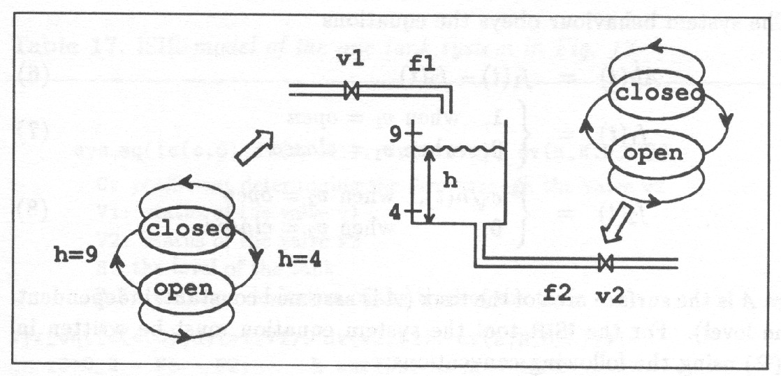
First an appropriate system specification is constructed. Some significant values of the system parameters are defined as landmarks.
qspace(h,[-100,0,4,9,100]).
qspace(_,[-100,0,100]).
qspace(Id, Landmarks)
Id:
the identifier of the variable
Landmarks:
ordered list of the landmarks
In the ISIR approach the state space is divided into discrete regions and the initial landmarks provide a discretization to be completed by the algorithm. 0 is generally a significant threshold value and it is thus defined as a landmark value for all the variables. and are also generally significant values. However, here and would be used only to designate values outside the normal range of operation, i.e. to designate the ranges and . Thus and can be replaced with any values clearly outside the intended range of operation of the system. In the current system for example and are clearly outside the normal range of any of the variables. 4 and 9 are significant threshold values for the level. The quantity space is specified with a set of predicates qspace as shown in Table 161010Constraint logic programming language CLP() is used in writing the specifications..
The system behaviour obeys the equations
| (6) | |||||
| (7) | |||||
| (8) |
where is the surface area of the tank ( is assumed constant, independent of the level). For the ISIR tool the system equation must be written in CLP() using the following conventions:
-
•
The system model is represented as a predicate sys_eq
sys_eq(XX)
-
XX:
list of state variables and system parameters
-
XX:
-
•
Constants in XX are represented as structures
c(Id,X)
-
Id:
the identifier of the constant
-
X:
the value of the constant
-
Id:
-
•
Discrete variables are represented as structures
dv(Id,X)
-
Id:
the identifier of the variable
-
X:
the value of the variable
-
Id:
-
•
When a point in the state space is determined the values of the variables and their derivatives are given directly using real numbers. Such continuous-time variables are represented as structures
cv(Id, Magnitude, Derivative)
-
Id:
the identifier of the variable
-
Magnitude:
the magnitude of the variable
-
Derivative:
the value of the time derivative of the variable
-
Id:
-
•
When the values are used to represent a region in the state space, they must tell the upper and the lower limit of the value or tell that the variable has a point value (representing an interval of zero length). Such values of state variables are represented as structures
i(Low, High)
-
Low:
lower limit of the value
-
High:
higher limit of the value
or as a structure
p(X)
-
X:
value of the variable
representing an interval or a point value, respectively.
-
Low:
-
•
Model equations are represented as CLP() constraints. Normal Prolog conventions are used in representing the relations between symbolic values.
sys_eq([c(c,C),dv(v1,V1), dv(v2,V2),cv(h,H,D_H)])
- C:
coefficient determining the flow through the valve v2
- V1:
status of the valve v1
- V2:
status of the valve v2
- H:
the level of the tank
- D_H:
the time derivative of the level of the tank
sys_eq([c(c,C),dv(v1,V1), dv(v2,V2), cv(h,H,D_H)]):-
   10*D_H = F1 - F2,     % surface area = 10m2
   fin(V1,F1),
   fout(C,V2,H,F2).

fin(open,1).
fin(closed,0).

fout(_,closed,_,0).
fout(C,open,H,Fout):- Fout*Fout = C*C*H, Fout = C*pow(H,0.5).
Because CLP() cannot solve from the equation an explicit solution is given. In general, if is the only nonlinear constraint in the model, having both and in the model guarantees that the problem can be solved whichever is known, or .
An initial state is specified for the system: .
init([c(c,i(0.3,0.4)),dv(v1,closed), dv(v2,open),cv(h,p(9),_)]).
In the ISIR-algorithm dynamic properties of the system are analyzed by applying ‘rules’ based on the intermediate value theorem telling how a continuous time function behaves. For example if and then at some later time it must be either or . When constructing these rules the time axis is assumed to consist of time intervals separated by time points, at which some significant change occurs for one or more of the system parameters. Thus, continuous change is represented with episodes during which the function is smoothly increasing, decreasing or steady and with significant changes occurring at time points separating these episodes.
The continuity rules are built into the ISIR-algorithm and they will be discussed later. The analysis of the continuous change is based on the sys_eq specification which tells the relation between system state variables and their derivatives.
The discrete control actions taken by the automatics or the operator cause a significant change thus justifying the current time interval to be broken by a time point. The discrete control actions have a separate specification. Here only the control system has discrete dynamics but in general also the plant can be modelled to have some discrete dynamics. Control actions are assumed to be taken instantaneously at a time point according to the following specification:
| (9) | |||||
| (10) | |||||
| (11) | |||||
| (12) | |||||
| ! error ! | (13) |
The specifications of the transitions of are a straightforward translation of the logic diagrams in Fig. 17. When the level reaches the value valve must be opened, when it must be closed. When the valve is left in its current position.
Because ISIR is partially based on the closed world assumption1111Closed world assumption means that the relations describing the state of affairs define explicitly or implicitly everything that can be true. If there are only two definitions for the relation f, f(a,b) and f(a,c), then under the closed world assumption it can be deduced that a and d are not in relation f, i.e. f(a,d) is false. Without the closed world assumption the truth value of f(a,d) could not be deduced. The closed world assumption is often used for pragmatic reasons. It is important to realize that the closed world assumption does not require that the model should describe the system behaviour explicitly. However, it means that an erroneous model may prevent some behaviours from being revealed when using the current ISIR-prototype., the specification must introduce all the possible characteristics of the behaviour. Thus, it is necessary to explicitly state something about undesired states as well because otherwise they would be considered inconsistent with the model. One possibility is to give an error message if the level exceeds the normal limits1212Currently the completeness of the specification is the responsibility of the specifier, which of course violates the very principle of verification. However, it is simple to make a separate tool which checks the completeness of the specification. For example, the left hand side of the above specification must cover both the cases where the valve is either open or closed for all the values of h..
The specification d_trans in Table 18 simply lists the relations between the current state of the valve, the condition triggering a transition, and the new state. For those situations where there is no change the relation tells that the old and the new values are the same. Such specifications can be generated automatically from logic diagrams.1313Automatic generation of such specifications is not implemented in ISIR.
The predicate d_trans collects the specifications of the operations of the valves together. It also specifies which state variables remain unchanged when the valves are opened and closed and which may change. Because opening and closing the valves may cause discontinuity in it is allowed to experience an abrupt change at time points.
d_trans([C0,U10,U20,cv(h,H0,_)],[C0,U1,U2,cv(h,H0,_)],
     [_,U1_tr,U2_tr,_]):-
     v1_tr(cv(h,H0,_),U10,U1, U1_tr), v2_tr(U20,U2,U2_tr).

v1_tr(cv(h,p(4),_),_,dv(v1,open),bb).
v1_tr(cv(h,p(9),_),_,dv(v1,closed),cc).
v1_tr(cv(h,i(L,H),_),V1,V1,aa):- 4 <= L, H <= 9.
v1_tr(cv(h,p(X),_),V1,V1,aa):- 4 < X, X < 9.

v1_tr(cv(h,i(L,H),_),V1,V1,aa):-
     (L < 4; H > 9), writeln('level exceeded').
v1_tr(cv(h,p(X),_),V1,V1,aa):-
     (4 > X; X > 9), writeln('level exceeded').

v2_tr(dv(v2,open),dv(v2,closed),bb).
v2_tr(dv(v2,closed),dv(v2,open),cc).
v2_tr(V2,V2,aa).
The above specification is sufficient to determine which states the system can reach from the initial state. Fig. 18 gives one of the outputs of the analysis obtained with ISIR. It shows the reachability graph of the qualitatively different states which the system can reach. The longer edges indicate time intervals and the shorter edges indicate the instantaneous discrete changes.
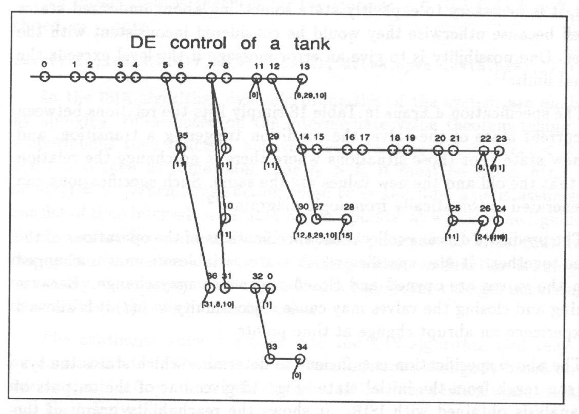
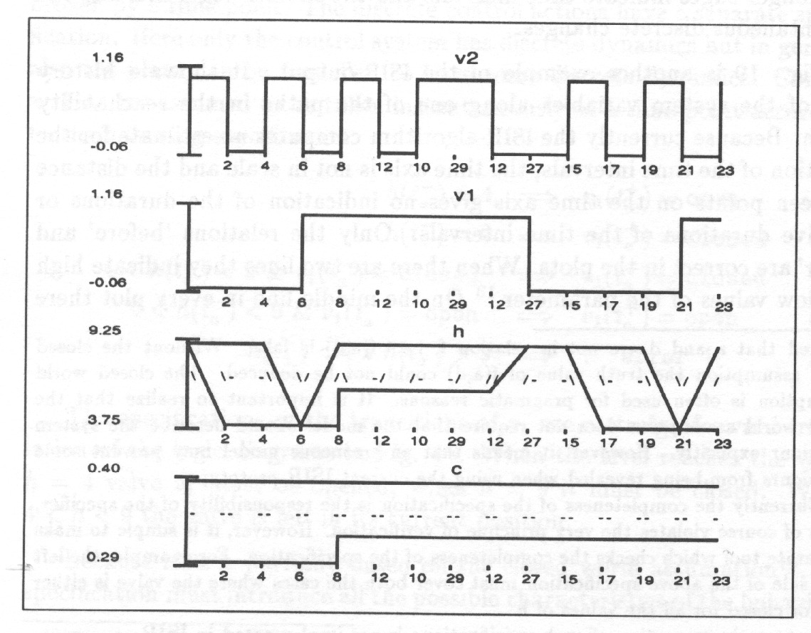
Fig. 19 is another example of the ISIR-output. It shows a history plot of the system variables along one of the paths in the reachability graph. Because currently the ISIR-algorithm computes no estimate for the duration of the time intervals, the time axis is not in scale and the distance between points on the time axis gives no indication of the durations or relative durations of the time intervals. Only the relations ‘before’ and ‘after’ are correct in the plots. When there are two lines they indicate high and low values of the parameter.1414Actually the high and low values at the time points are simply connected with straight lines or second order curves. So the plots do not represent accurately the envelopes of the actual behaviours. On the middle line in every plot there are markers ‘/’, ‘–’ and ‘’ indicating that the parameter is increasing, steady or decreasing respectively.
In addition to the plots individual states and state transitions can be studied in detail. For example the changes occurring at state 7 can be listed. In Table 19 the left column shows the ‘old’ values and the right column the ‘new’ values of the system state variables. The signs ‘’, ‘m’ and ‘d’ in the middle column tell if the variable remains unchanged, if its magnitude (and maybe derivative) is changed or if only its derivative is changed.
7 (p1) -> 8 (p0)
Id   magnitude     derivative    ->  magnitude      derivative
c:   0.3 - 0.4        0           m  0.333 - 0.4        0
v1:     open          0           =    open             0
v2:     closed        0           m    open             0
h:     4 - 9          0.1         m  6.25 - 9     -0.02 - 0

7 (p1) -> 9 (p0)
Id   magnitude      derivative   ->  magnitude      derivative
c:    0.3 - 0.4       0           =  0.3 - 0.4           0
v1:     open          0           =    open              0
v2:     closed        0           m    open              0
h:      4 - 9         0.1         d  4 - 9             0 - 0.04

7 (p1) -> 10 (p0)
Id  magnitude      derivative    ->  magnitude      derivative
c:   0.3 - 0.4       0            m  0.333 - 0.4         0
v1:    open          0            =    open              0
v2:    closed        0            m    open              0
h:     4 - 9         0.1          m  6.25 - 9            0
Table 19 tells that when and is open then opening may result in the level either increasing, decreasing or becoming steady, depending on the value of the parameter c. It also shows that only when the level is high enough is it possible that inflow is smaller than outflow when both of the valves are open.
In the previous analysis the constant parameter c has been allowed to obtain a smaller range of uncertainty during the prediction of the behaviour. This is justified as the predicted behaviour, the level not increasing, is possible only if the parameter c is large enough. However, it depends on the problem to be solved whether narrowing the range of constants is desired or not. ISIR can be modified to treat the constants in a desired way. Whichever option is chosen, ISIR will always consider the possibility that the minimum or the maximum of some of the variables is not obtained at the limits of constant parameters.
Some analysis could be based on conventional quantitative simulation. However, here the goal is to find all the significantly (qualitatively) different behaviours, and the results of the analysis are meant to be used in automated reasoning. To find all the significantly different behaviours or accessible states with simulation only would require complex computations. Because the valve parameter is not known exactly, some kind of Monte Carlo simulation would be necessary. Because the timing of the operation of the valve is not known, it should be opened and closed at random intervals during the simulation requiring a lot of computation and still falling short of giving full guarantee that all the possible behaviours are revealed. The 37 states and the transitions between them can be used more efficiently in automated problem solving than the data generated by Monte Carlo simulation.
Although in this example the future behaviour is predicted when the control algorithm is specified, very often it is necessary to do the opposite, find control actions which result in a satisfactory plant behaviour.1515It is important to notice the difference between the nature of stabilizing continuous-time control like PID-control and optimal control; discrete-event control strategies like automatics, operating procedures, interlocks and protections.
Altogether it is evident that much of the analysis and synthesis of discrete-event control is logic reasoning and that it is sufficient to know whether the tank level is between the limits 4 and 9, above 9 or below 4 and whether it is increasing, decreasing or steady. For example when the level is increasing, nothing interesting happens until the level is reached or the states of valves are changed. Thus, it is unnecessary to predict the behaviour of the level in any more detail between those events.
In general it is not important to know what the rates of change are but in which order the significant events may occur. For example to predict how long it takes to fill a tank actually requires exact knowledge on the characteristics of the liquid, of the valves etc. Control strategy based on such an exact model may lack robustness. System time constants and consequently the order of the occurrence of some critical events may change when a valve is changed, the characteristics of the liquid change, or the control sequence is initiated when there is some liquid left in the tank. To guarantee robustness the design must be based on ranges of system parameters, not on one single set of parameters.
4.2.1 Analysis of the reachability graph
The output presented in the previous section is produced for visualisation of the behaviour of the system. However, the mechanised problem solving applied in the analysis and synthesis of the control systems is more important. Some simple examples on using the state graph are given, although many problems can be solved also without generating the whole state graph.
st(p0,0,[c(c,i(0.3,0.4)), dv(v1,closed), dv(v2,open),
   cv(h,p(9),i(-0.12,-0.09))]).
st(p1,1,[c(c,i(0.3,0.4)), dv(v1,closed), dv(v2,open),
   cv(h,i(4,9),i(-0.12,-0.06))]).
st(p0,2,[c(c,i(0.3,0.4)), dv(v1,closed), dv(v2,closed),
   cv(h,i(4,9),p(0))]).
st(p1,3,[c(c,i(0.3,0.4)), dv(v1,closed), dv(v2,closed),
   cv(h,i(4,9),p(0))]).
 . . .
tr(0, 1).
tr(1, 2).
tr(2, 3).
tr(3, 4).
tr(4, 5).
 . . .
The reachability graph is stored in a file as a set of Prolog predicates. Predicates
st(TpTi,No, XX)
- TpTi:
time index telling the start points of episodes form the end points
- No:
id. number of the state
- XX:
system state as a list of state variables
specify the states while predicates
tr(X, Next_X)
- X:
Id. number of a state
- next_X:
Id. number of the successor of X
specify the transitions. Table 20 shows part of the graph in Fig. 18.
Thus, the graph is a Prolog program and it can be analyzed in a straightforward manner. In principle the truth value of any temporal logic theorem can be checked. As a simple example it is possible to search for the states which have no successors.1616Dead-lock in a discrete-event system is a typical example of such a state. The predicate dead_end in Table 21 goes through the state graph and reports all the states which have no successors. Most systems should have a cyclic behaviour and thus dead-ends can be considered as indications of an error either in the model or in the system design.
dead_end:-
   st(_,B,_),                 % there is a state B
   (tr(B,_)                   % if there is a transition further
      -> fail                 %    then reject B
      ; format('~w;  ',[B])), %    else report a dead-end
    fail.                     % backtrack for all other states
Dead-ends in the graph can be listed simply by calling dead_end:
| ?- dead_end.
no
As another example, it is possible to search for situations where both the valves are open and the level still remains stable, see Table 22
stable:-
     st(_,B,[c(c,C),dv(v1,open), dv(v2,open),cv(h,H,p(0))]),
     format('state: ~w  c: ~w  h: ~w~n ',[B,C,H]),
     fail.

?- stable.
state: 10  c: i(0.333333,0.4)  h: i(6.25,9)
state: 11  c: i(0.333333,0.4)  h: i(6.25,9)
no
4.2.2 Synthesis of a control sequence
d1_trans([C0,U10,U20,cv(h,H0,D_H0)],[C0,U1,U20,cv(h,H0,D_H)],
         [_,_,_,_]):-
  control(H0,D_H0,D_H,U10,U1).

control(H0,D0,D1,_,_):- gte(H0,p(9)), !, zerneg(D1), gte(D0,D1).
control(H0,D0,D1,_,_):- gte(p(4),H0), !, zerpos(D1), gte(D1,D0).
control(_,_,_,X,X).

gte(p(X),p(Y)):- X >= Y.
gte(i(X,_),i(Y,_)):- X >= Y.
gte(i(X,_),p(Y)):- X >= Y.
gte(p(X),i(_,Y)):- X >= Y.

zerneg(p(X)):- X <= 0.
zerneg(i(_,H)):- H <= 0.

zerpos(p(X)):- X >= 0.
zerpos(i(_,H)):- H >= 0.
In the previous example the control sequence of Fig. 17 was verified. Very much the same approach can be used to support the synthesis of a control sequence. Instead of specifying the conditions under which the valve should be operated, the conditions that should be true can be specified as show in 23 The discrete transition of Table 18 is divided into two simultaneous transitions from which d1_trans represents the control actions. The only variables that are allowed to change are U10 U1 and D_H0 D_H. (I.e. input valve can be manipulated with a possible result of the derivative of the tank level obtaining a new value. Further, the valve is allowed to change status only when the level is or . In those cases it is required that the derivative of the tank level is such that the level is moving towards the acceptable region. When is open the level decreases even when is open. This is acceptable but to get a better result it is further required that if the status of is changed the change must result in the level moving faster towards the desired region.
The program in Table 24 can be applied on the resulting state graph to identify the conditions under which the control actions are needed.
synth:-
    st(p1,B,Sb),
    tr(B,C),
    st(p0,C,Sc),
    action(Sb,Sc,Str),
    tr(A,B),
    st(p0,A,Sa),
    nl,
    wr_synth(Sa,Sb,Str),
    fail.

action([_,dv(v1,V1b),_,_],[_,dv(v1,V1c),_,_],(V1b,V1c)):-
dif(V1b,V1c).

wr_synth([_,_,_,Ha],[_,_,_,Hb],(V1b,V1c)):-
    write(Ha),write(' -> '), write(Hb),write(': '),
    write(V1b), write(' -> '), write(V1c),nl.
| ?- synth.
cv(h,i(4,9),i(-0.12,-0.06))
  -> cv(h,p(4),i(-0.08,-0.06)):   closed -> open
cv(h,i(4,9),i(-0.12,-0.06))
  -> cv(h,p(4),i(-0.08,-0.06)):   closed -> open
cv(h,i(6.25,9),p(0.1))
  -> cv(h,p(9),p(0.1)):             open -> closed
cv(h,i(4,9),p(0.1))
  -> cv(h,p(9),p(0.1)):             open -> closed
cv(h,i(6.25,9),p(0.1))
  -> cv(h,p(9),p(0.1)):             open -> closed
cv(h,i(4,9),p(0.1))
  -> cv(h,p(9),p(0.1)):             open -> closed
cv(h,i(4,9),i(-0.12,-0.0667))
  -> cv(h,p(4),i(-0.08,-0.0667)): closed -> open
cv(h,i(4,9),i(-0.12,-0.0667))
  -> cv(h,p(4),i(-0.08,-0.0667)): closed -> open
cv(h,i(4,9),p(0.1))
  -> cv(h,p(9),p(0.1)):             open -> closed
cv(h,i(4,9),p(0.1))
  -> cv(h,p(9),p(0.1)):             open -> closed
no
| ?-
The result in Table 25 can be used to help in constructing the control sequence: The valve must be opened when the level reaches the low limit and it must be closed when the level reaches the high limit.
4.2.3 Control requirements specified with a state automaton
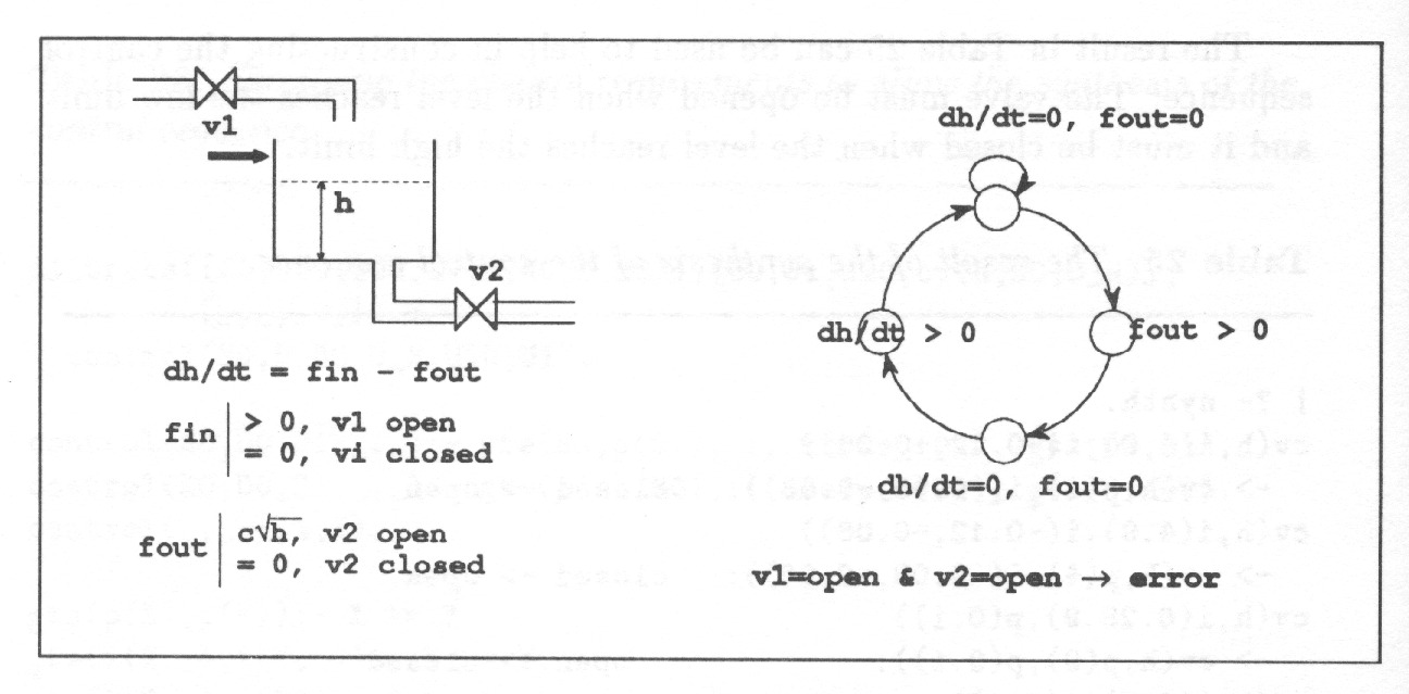
It is common to specify the control requirements with a state automaton sketching the desired behaviour of the overall system as shown in Fig. 20. The specification of the systems and the control requirements are given in Table 26.
sys_eq([dv(stp,Stp),c(c,C), dv(v1,V1),
dv(v2,V2),cv(h,H,D_H)],_,[]):-
        10*D_H = Fin - Fout,  % surface area = 10m2
    fin(V1,Fin), fout(C,V2,H,Fout),
    control(Stp,Fout,D_H),
    legal_v(V1,V2).

/*  the conditions which should be true in all states */
control(1,0,0).     % Rest state
control(2,Fout,_):- % Liquid has been demanded.
    Fout > 0.       % There must be outflow
control(3,0,0).     % Wait to be sure that only one valve is
open
control(4,_,D_H):- D_H > 0. % Fill the tank

legal_v(closed,closed).
legal_v(closed,open). % Never open both valves simultaneuously
legal_v(open,closed).

/* Some mechanistic work is needed to make the following less
awkward.

There are often two alternatives: no change or jump to the next
step.
The tank level determines the jumps, or it occurs
spontaneously, or it is forced to take place.*/

d_trans([dv(stp,1)|S], [dv(stp,1)|S],_).
d_trans([dv(stp,1),c(c,C),dv(v1,_), dv(v2,_),cv(h,p(9),_)],
    [dv(stp,2),c(c,C),dv(v1,_), dv(v2,_),cv(h,p(9),_)],_).

d_trans([dv(stp,2),c(c,C),dv(v1,_), dv(v2,_),cv(h,i(L,H),_)],
    [dv(stp,2),c(c,C),dv(v1,_), dv(v2,_),cv(h,i(L,H),_)],_):- H
> 4.
d_trans([dv(stp,2),c(c,C),dv(v1,_), dv(v2,_),cv(h,p(4),_)],
    [dv(stp,3),c(c,C),dv(v1,_), dv(v2,_),cv(h,p(4),_)],_).

d_trans([dv(stp,3),c(c,C),dv(v1,_), dv(v2,_),cv(h,p(4),_)],
    [dv(stp,4),c(c,C),dv(v1,_), dv(v2,_),cv(h,p(4),_)],_).

d_trans([dv(stp,4),c(c,C),dv(v1,_), dv(v2,_),cv(h,i(L,H),_)],
    [dv(stp,4),c(c,C),dv(v1,_), dv(v2,_),cv(h,i(L,H),_)],_):- L
< 9.
d_trans([dv(stp,4),c(c,C),dv(v1,_), dv(v2,_),cv(h,_,_)],
    [dv(stp,1),c(c,C),dv(v1,_), dv(v2,_),cv(h,p(9),_)],_).
The resulting behaviour can be seen in Fig. 21.
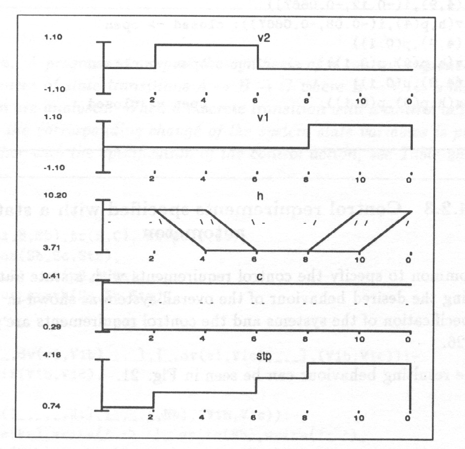
4.2.4 Proportional control of the tank level
Because the discrete-event control system often manipulates the stabilazing continuous-time controllers ISIR must handle such systems properly. If valve is a control valve the discrete feedback of the previous example can be replaced with continuous feedback control as shown in Fig. 22.
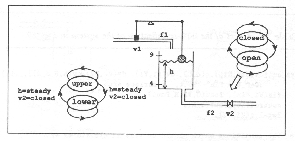
In the example it is assumed that there are two modes of operation, one having the controller setpoint at 6m and the other having the setpoint at 4m. A different feedback coefficient is also used. The mode of operation is assumed to be changed by the operator only when the valve is closed and the level has stabilized to its reference.
To take into account the saturation of the controller — negative inflow is not allowed — the system specification is divided into two as shown in Table 27.
sys_eq([c(c,C), dv(moodi,Moodi), dv(v2,V2),cv(h,H,D_H)],_,Frz):-
   fin(Moodi,K,R), R >= H,
   10*D_H = K*(R-H) - C*V2*pow(H,0.5),
   sec_ord(K,C*V2,10*D_H-K*R,Z,Frz),
   Z*Z = H.
sys_eq([c(c,C), dv(moodi,Moodi), dv(v2,V2),cv(h,H,D_H)],_,[]):-
   fin(Moodi,_,R), R < H,
   10*D_H = -C*V2*pow(H,0.5),
   (V2 > 0 -> H = pow(-10*D_H/C/V2,2); true).

fin(upper,0.2,6).
fin(lower,0.25,4).

d_trans([C0,U10,U20,cv(h,H0,_)],[C0,U1,U2,cv(h,H0,_)],
         [_,U1_tr,U2_tr,_]):-
   mode_tr(cv(h,H0,_),U20,U10,U1, U1_tr), v2_tr(U20,U2,U2_tr).

mode_tr(_,_,Moodi,Moodi,aa).
mode_tr(cv(h,p(6),p(0)),dv(_,0),dv(moodi,upper),
        dv(moodi,lower),ba).

v2_tr(V2,V2,aa).
v2_tr(dv(v2,1),dv(v2,0),ba).
v2_tr(dv(v2,0),dv(v2,1),ab).
Fig. 23 shows the state graph generated with the specification when the depth of the graph is limited. Fig. 24 shows that the proportional controller takes the level exactly into the reference when there is no outflow, otherwise there is a deviation but the level is always kept between the acceptable limits.
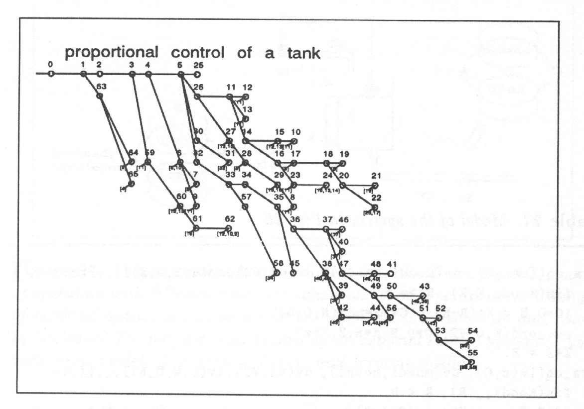
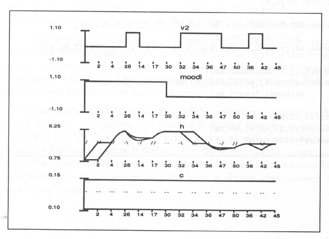
Summary
Because there are discrete features in process plant controlstrategies, techniques of discrete mathematics used e.g. in computerscience can be applied. However, they fall short in treating continuous time systems. Qualitative modelling provides many principles on how to fill this gap, but they must be modified to suit for solving control problems. Logic programming and especially constraint logic programming languages seem to be the best choice to implement tools required in the analysis and design of such systems.
4.3 SUBTASKS IN MODEL-BASED REASONING
The ISIR-algorithm is implemented with the constrain-and-generate approach which allows describing the problem domain as a set of generators defining the problem space and as a set of constraints differentiating acceptable solutions from unacceptable ones. Reasoning based on a plant model is divided into implementing the following relations:
- consistent state:
-
1717In Fig. 10 this task corresponds to determining which values of and are consistent in any of the states.
System model is represented as
(14) (15) Relation ‘consistent state’ checks that the values of the variables are always consistent with the model. It also solves the unknowns as well as possible.
Mathematically this is a constraint solving problem where the constraints — mathematic equations and inequalities and logic axioms — tell the relationships between the system variables.
Determining a consistent state can be used as such to solve some low-level problems like: “How to make the temperature T increase?”; “how to make the steam flow from tank A to tank B?”; “is it possible that level h is decreasing although valve V is closed or has some fault occurred?”
- consistent transition of a variable:
-
There are two kinds of transitions,
- :
-
the evolution of the continuous time variables during an episode;
- :
-
Instantaneous discrete changes; for example an automatic control sequence taking a step. Discrete changes may also change the derivatives of the continuous time variables.
Possible transitions of a variable are determined or it is checked that a given transition is in accordance with the related constraints.
- consistent state transition:
-
Determine transitions of the system state which are consistent with the system model and the additional constraints. This is accomplished by applying the conjunction of the above two relations.
of the pairs of each
variables are constraint. For discrete given directly
- behaviours:
-
Applying recursively the above gives a state graph representing all the possible behaviours of the system.
behaviour. required to transition a state
Having the state graph it is possible to solve problems like “how to take the plant into a state which satisfies the following conditions: …?”. At this level some principles of modal logic or temporal logic must be adopted in reasoning.
- planning:
-
The above state and transition constraints can be used as the domain model in solving various planning problems. In planning it is in addition necessary to have the specification of the goal of operation.
- verification:
-
Verification of the plant automatics can be based on the above. For example as a brute force approach a complete state graph representing the behaviours can be generated and searched for undesired properties.
In the following the above is discussed in more detail. Algorithms in Prolog and CLP() are used to illustrate the central parts of a principal solution to the reasoning problem. However, not all of those pieces of programs correspond exactly to the actual ISIR-algorithm.
4.3.1 Consistent states
At any time point or during any time interval the value of any variable or its derivative is either known, unknown or partially known. For example, real-valued variables may be constrained into an interval, and discrete variables may be constrained in having a small set of alternative values. One of the low-level problems is to solve some of the variables when others are (partially) known. For continuous-time variables also the direction of change must be determined.
Part of the model is represented as logic axioms. Problems related to this part can be solved with mechanised logic reasoning as implemented for example in the programming language Prolog. The rest of the model contains mathematical equations and inequalities. Because ISIR is implemented in CLP() it can directly solve mixed logic-numeric problems.
Often the values of the variables and model parameters can be given as numerical intervals and the relationships between them as mathematical equations. Then the smallest hypercube in the state space which contains all the possible solutions to the model equations can be considered as a state consistent with the constraints. Determining such a hypercube is an optimisation problem:
| (16) |
When is linear, the problem can be solved with linear programming. Because typically is nonlinear, an algorithm to solve nonlinear problems is developed. The algorithm shown in Table 28 directly applies the principles presented in section 3.7. A predicate f(X) is needed to implement and predicate corners(LH,X) is needed to give the values
for all the one by one. The predicate local_extrem is used to determine local extremes, e.g. the points where partial derivatives of any of the variables vanish. Finally, it is necessary to search for the minimum and the maximum of each variable1818The piece of code in Table 28 is a slightly simplified version of the actual ISIR-algorithm, but it correctly reflects the actual principle..
extrema(LHa,LHb):-
   tell('tmp.tmp'),
   f(X),
   low_high(closed,X,LHa),
   corners(X, LHa),
   local_extrem(X),
   ground(X),
   printf('xx(%).\n',[X]),
   fail.
extrema(LHa,LHb):-
  told,
  see('tmp.tmp'),
  search_limits('tmp.tmp', LHb).
It is also checked that there is an interior point in the region which satisfies the equation constraints. This is done for efficiency reasons to check if there is inside the region a point which satisfies the given conditions before starting to search the borders of that region. The other reason is that the predicate extrema may succeed in finding the borders of a region even though there is not a single point satisfying the conditions inside the region.
The interior point is searched with a predicate similar to extrema but the predicate corners(X,LHa) is replaced with the predicate interior_point(X, LHa) giving X the following alternative values
| (17) |
until a solution to the system equation is found.
Choosing the state variables
The state vector is defined to be the set of variables which, together with the external input vector, gives all the information necessary to determine the future behaviour of the system. For example, the system equation for a mass-spring system with friction can be written as . The state variables are and which uniquely determine the direction of the change at any point in the plane and thus are sufficient to determine the future of the system. However, in ISIR the state is typically defined, like for example . Then it is not even known whether which indicates that it is useful to include into the state vector. This is why in ISIR (and also in QSIM) the derivatives of the state variables are included into the state vector1919For example in QSIM all the variables used in the constraints in the model are treated as state variables, and due to operations mainly on triples and pairs, this results in all the intermediate variables to be included into the state vector. In ISIR this is not the case: In complex models not all the intermediate results are explicitly computed. ISIR-models can be given a modular structure so that it may be difficult to pass all the intermediate results from all the subroutines and functions used in modelling..
In the above case it is useful to take also the second derivative of a variable into the state vector. (In the above example that would occur automatically in QSIM).
For the problems encountered when applying the ISIR-algorithm, it is useful to discretize the state space so that the zeroes of the gradients, lie outside or on the borders of the region under consideration. When , the region can be divided into three; and , so that , and . If ,where is a subvector of with dimension higher than one, then an auxiliary variable is used.
However, ISIR can also handle cases where there are extrema inside the region under consideration. Thus the above is not necessary but may sometimes help in pruning the solution space during the synthesis of the behaviours of the system.
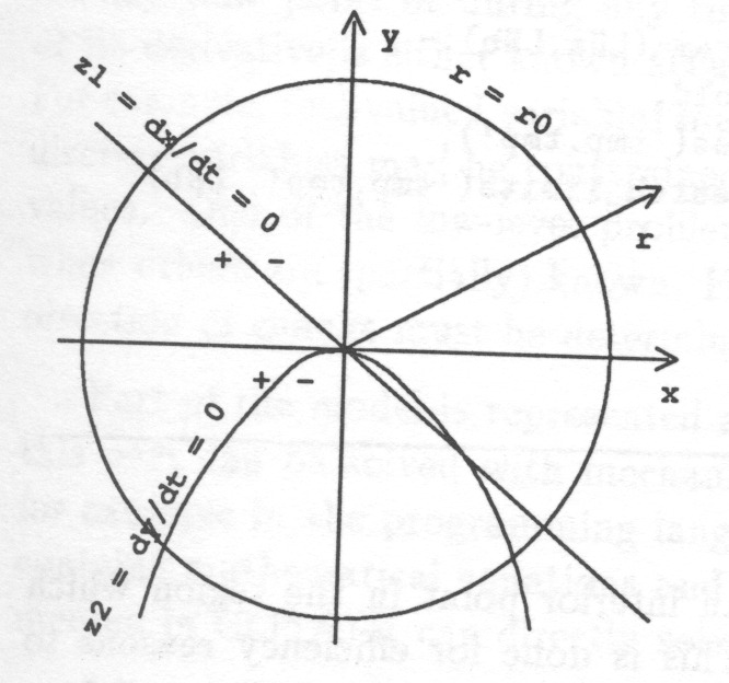
Auxiliary variables other than the derivatives can also be included into the state vector. When using real values a sum of n independent vectors spans an n-dimensional space. However, when using intervals the situation is different as shown in Fig. 25. On a two-dimensional rectangular coordinate system intervals of the coordinates define a rectangle. If only the signs of the derivatives are taken into account nine directions can be distinguished. Additional variables, like can be used to tighten the division of the state space and the possible directions of change.
Additional auxiliary variables do not help in pruning the behaviours if there are no additional constraints on the auxiliary variables. For example, making energy an additional state variable does not as such help in pruning the behaviours. But if it is possible to say something about the conservation of energy this will constrain the behaviours.
4.3.2 Consistent change of continuous functions
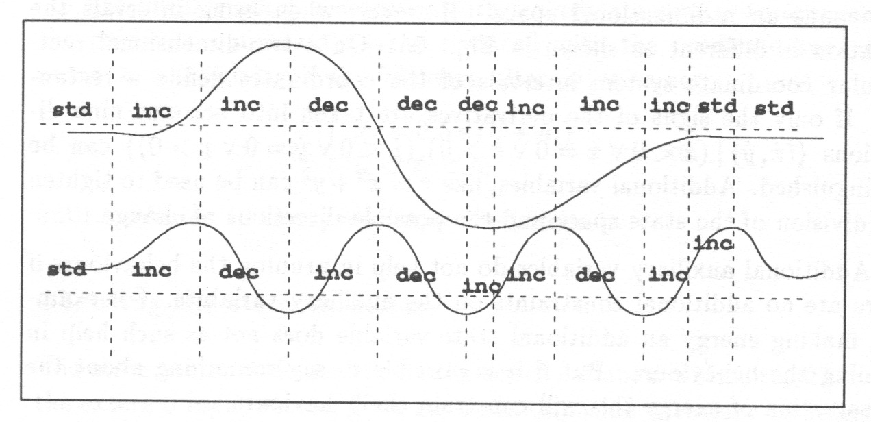
The first step in analyzing the dynamics of the model in terms of the discrete-event paradigm is to determine possible state transitions from one state to the next one. To do this the possible changes of the variables must be defined. For discrete variables such an accessibility relation can be determined directly in cases typically encountered in plant automatics, because it is possible to list one by one the possible changes of the individual variables and the preconditions for those changes.
For discretized continuous-time variables, the changes in the values occur when crossing some significant limits or when the sign of the derivative changes. The behaviour of a continuous time function between two significant time points and can be characterised using the values of the function and sign of its derivative at the end points and of the time period if it is assumed that neither the first nor the second order derivative change sign during the period. Fig. 26 shows the division of the system behaviour into episodes according the the signs of the first oerder derivatives only.
Fig. 27 shows three of the seven alternative shapes of a continuous time function between two significant time points. The fourth is the steady behaviour and the three remaining are the decreasing counterparts of the increasing ones.
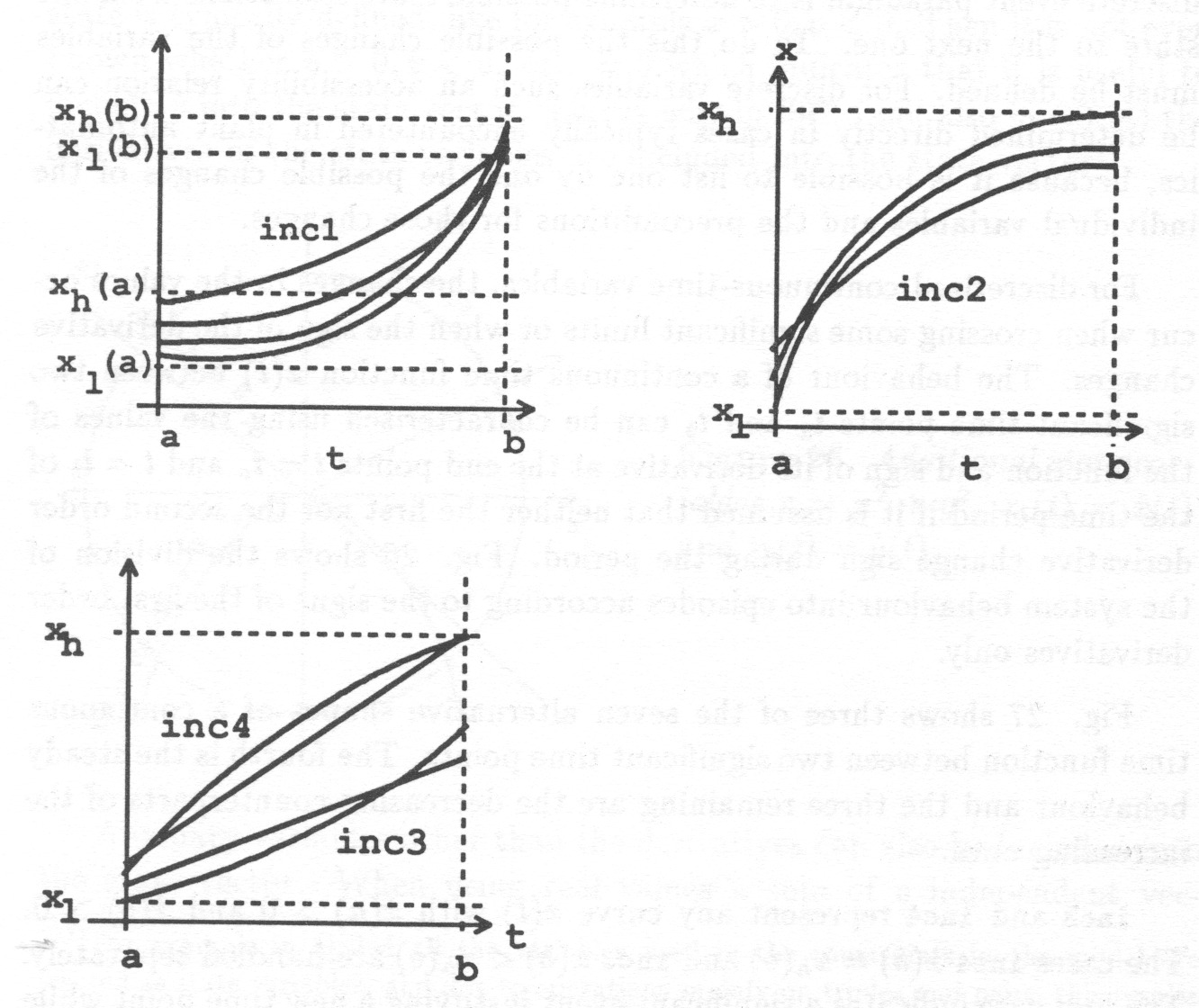
inc3 and inc4 represent any curve with and . The cases inc4 and inc3 are handled separately. The first case indicates a significant event justifying a new time point while the second does not.
Intermediate value theorem of equation 18 can be used in writing constraint equations defining the different possible shapes of the functions during an episode.
| (18) |
Equation 19 is a constraint telling if the function can have a behaviour of the type inc1 between time instants and . Constraint 20 tells the range of possible values for including the upper and the lower limit of the range. 19 is used to check if an episode of type inc1 is possible and 20 is used in constraining the acceptable values of .
| (19) | |||||
| (20) | |||||
where and are the prior upper and lower limit of .
| (21) | |||||
| (22) | |||||
The second order derivative or is used only at points where the first order derivative vanishes, for example at the beginning of an episode of type inc1 or at the end of an episode of type inc2. The condition in the equation 21 is not strictly in accordance with the properties of continuous functions. The equality allows asymptotic approach of a stable behaviour to be treated as if it occurs in a finite time. If needed, the two cases reaching a turning point and asymptotic approach to a stable point, can be separated.
The algorithms in the previous section are used to determine the constraints for the upper and the lower limit of . Table 29 shows as an example how the transition constraint of equation 19 is actually implemented.
tr(TrCode,Xa, LHa, X, LH, Xb, LHb, DDa, DDb)
-
TrCode:
One of the strings std, inc1, inc2, inc3, inc4, dec1, dec2, dec3, dec4 telling the shape of the curve
-
Xa:
at
-
LHa:
The limits and at
-
X:
at
-
LH:
The limits and at
-
Xb:
at
-
LHb:
The limits and at
-
DDa, DDb:
and
tr(inc1,cv(Id,Xa,0),cv(Id,i(La,_),p(0)),
   cv(Id,X,DX),cv(Id,i(Xa,Xb),i(0,DXb)),
   cv(Id, Xb, DXb), cv(Id, i(La, Hb), i(0,#inf)), DDa,_):-
    upper(Id,La,Hb),
    Xa < X, X < Xb, Xb <= Hb,
    DX > 0, DXb > DX,
    DDa > 0.
upper(Id,X,H)
- Id:
The identifier of the variable
- X:
The value of the variable
- H:
The nearest landmark of Id, for which .
Proof of the Treatment of Continuous Change
Equation 19 is first discussed. Initially and are known. They form the generator base in this case.
According to intermediate value theorem 18 any smooth continuous function must satisfy the conditions given by the equation 18.
Thus 19 does not exclude any possible behaviour with the given initial conditions. Because there are alternative definitions for other initial conditions and other shapes of curves as well, no possible alternative is excluded. 20 does not exclude any possible solution.
However, it is not guaranteed, that all the impossible behaviours are excluded.
4.3.3 Consistent state transitions
Combining the constraints for a consistent state and those for consistent transitions of individual transitions results in a definition of a consistent state transition.
Consistent state transitions are determined with the same principle as when solving consistent states but now the state variables are loaded with additional transition constraints. The algorithm is presented in Table 30. The current state ( LHa) represents a region, a hypercube, in the state space. In effect ISIR computes points ( Xb) in the state space which obey the conditions determined by the definitions of the transitions for all the continuous variables ( trans) in addition to the conditions determining the mutual relations of the variables at the beginning, at the end and during the episode ( f(Xa,DDa), f(X,_), f(Xb,DDb)). These points are classified according to the transition labels ( TrC) to separate qualitatively different transitions. For all such classes of transitions the upper and lower limits of the variables and their derivatives ( LHb) are searched.
transitions(LHa,LHb):-
     tell('tmp.tmp'),
     low_high(open,Xa,LHa),
     f(Xa,DDa), f(X,_), f(Xb,DDb),
     trans(TrC,Xa,LHa,X,LH,Xb,LHb,DDa,DDb),
     low_high(closed,Xb,LHb),
     low_high(closed,X,LH),
     local_extrem(Xb),
     once(local_extrem(Xa),
          interior_point(Xb),
          interior_point(Xa),
          interior_point(X),
          ground([Xa,X,Xb])),
     printf('xx(%,%).\n',[Xb,TrC]),
     fail.
transitions(LHa,LHb):-
                      see('tmp.tmp'),
%search for the minimum and the maximum of each of
%the state variables for each of the transition codes
In transitions effective use is made of stepwise constraining of the solution to reduce backtracking and thus the complexity of the algorithm2020The actual algorithm is slightly more complex and somewhat different.. low_high(open,Xa,LHa) constrains initial state so that . f(Xa,DDa), f(X,_), f(Xb,DDb) constrain , and , to obey the system equations. trans calls recursively tr introduced in the previous section to make all the continuous state variables in , and obey the continuity rules. Then the two calls to low_high instantiate the variables in the state vectors and to either the upper or lower limit determined by trans or they are constrained in the open interval between the upper and the lower limit. local_extrem(Xb) instantiates into a local extrem of in case is not yet ground. Finally, points and which satisfy all the constraints are searched for.
The predicate transitions gives as les in every category must be determined. The classification is done simply according to the transition codes provided by the trans-predicate. Discussing the implementation of this part of the ISIR-algorithm is beyond the scope of this report.
The verification procedure proposed in section 3.2 reveals no errors2121Only the top level of the algorithm is discussed here.:
-
1.
Check that the generator base contains all the actual solutions.
The predicate trans calls recursively the continuity constraint tr giving a priori upper or lower limit for each depending on the shape of the episode. tr provides definitions for all the possible shapes.
low_high tries to instantiate each of the variables in turn into one of the values thus going through all the corners of the allowable space. local_extrem tries to instantiate the state into a value where any of the partial derivatives vanish. interior_point gives a value for the remaining uninstantiated variables. Thus all the possible extremes of are included.
-
2.
Check that the constraints do not exclude any solutions.
- low_high(X,LH)
-
Constrains the state vector X to lie in the closed region LH. Thus it does not exclude any solution.
- f(X,DD)
-
Because predicate f is the model equation it defines what the solution is. However, if there are nonlinearities in the equations, it may happen that the modeller fails to write such an explicit solution to the equation as to instantiate the variables sufficiently. Even in such a case no solution is actually excluded, but some are not identified, giving the same incorrect result.
- trans
-
Discussed earlier.
- interior_point
-
Discussed earlier.
- local_extrem
-
Discussed earlier.
-
3.
Check that the constraints exclude all the non-solutions.
f is part of the definition of the solutions. trans may generate some superfluous transitions. Thus ISIR, as QSIM, may generate superfluous solutions. This is due to the way the transition rules deal with the continuous change of interval variables.
-
4.
Check that the computation will end.
The computation will end if f and trans give only a finite number of alternatives. f is mainly a set of equations and trans is checked both manually and through various tests to give only a finite number of solutions.
-
5.
Explain the reason of using assert, retract, cut, if-then-else structures and other non-logical features.
The resulting points are written in a file. (Could be asserted as well). This is because generate-and-fail approach is used for efficiency reasons.
-
6.
If dynamic predicates are used, check that they are properly initialised.
None used.
-
7.
List the special assumptions on e.g. initial instantiation of the variables.
The current state, LH0, must be fully instantiated, because the algorithm is based on distinguishing the extremes by checking if the state is ground.
Employing numerical integration
The predicate tr which gives the continuity rules defines partially initial and final values for the continuous state variables and their derivatives. In addition it requires that the derivative of the variable must have the same sign during the whole episode. The predicate trans called in transitions applies tr on all the continuous state variables. The objective is to find minimum and maximum value for each under all the constraints. This is a two-point boundary value problem which can be solved using numerical integration instead of the algorithm in Table 30 as will be shown in section 4.5.1. However, this alternative is not yet integrated into ISIR.
Determining the consistent transitions with numerical simulation would not change the basic algorithm in any way. Determining a transition would require more computation time, but in many cases there would be less spurious transitions and the predicted limits of the behaviour would be more accurate. Representing the behaviour of external inputs would require some rethinking. For example if and the current algorithm assumes that . However, if numerical integration is used to give a ground result, must be assigned a ground value at each integration step. In principle this results in an optimal control problem.
4.3.4 Consistent behaviours
A typical control problem can be stated as follows:
“Determine possible admissible paths from one state satisfying given initial conditions into another state satisfying given end conditions.”
The principle of determining the behaviours when the accessibility relation between the states is available is demonstrated in the following. In terms of logic programming initial conditions can be denoted as init(S), end conditions correspondingly as end(S). Accessibility relation between two states corresponding to the transition relation discussed in the previous section can be denoted as trans(S0,S1), and admissible states as admissible(S). Then the required path can be defined in Prolog as shown in Table 31.
trans(a,b).
trans(b,c).
trans(b,a).
trans(c,d).
trans(a,f).
trans(f,g).
trans(g,d).

init(a).
end(d).

path([S0|Path]):-
  init(S0),end(Sn),
  access(S0,Sn,Path,[S0]).
access(Sn,Sn,[],_).
access(S0,Sn,[S1|Path], Passed):-
  trans(S0,S1),
  admissible(S1),
  not(member(S1,Passed)),
  access(S1,Sn,Path,[S1|Passed]).

admissible(X):- not(X = c).

| ?- path(Path).
Path = [a,f,g,d]
Due to implementation issues the ISIR-algorithm is not implemented as in Table 31 but rather as the algorithm in section 3.3. For the purposes of this report it is irrelevant to discuss this part of the actual ISIR-algorithm in any more detail.
Finding a solution to a control problem in the above form is not always sufficient. A solution like the above is useful for off-line analysis, for example in verification of plant automatics. In principle, a knowledge-based control system based e.g. on the ISIR-algorithm can be used in on-line control, but in practice a more efficient and more easily implemented control algorithm is typically required. Such a control algorithm can be extracted from the solution obtained by ISIR in the following way. List the transitions in which reaches a landmark. They are candidates for preconditions of a state transition of the control sequence. Then list the transitions of the control variables . Those changes are the candidates for control actions to be taken by the control sequence.
4.3.5 Planning
The previously presented techniques can be used to support the designer of plant automatics and the operators of a process plant, but they are not sufficient for fully autonomous problem solving. To achieve autonomous accomplishment of higher level control tasks formal specification of the goal of operation and operational restrictions must be developed and the above can be used as the domain model in planning. The designer should be supported in constructing a task hierarchy. Every task in such a hierarchy should have
-
preconditions telling when it is possible to initiate the accomplishment of the task;
-
support conditions telling what successful accomplishment of the task requires;
-
end conditions telling what the state of the affairs after the accomplishment of the task is.
In addition domain-specific ways to let the human designers characterize their beliefs on what a good solution is like should be developed. There should be application-oriented primitives to constrain the search space and to give priorities to alternative search paths.
Some problem specific descriptions of the desired behaviour have been made but the ISIR requires modifications to make them generally applicable.
4.3.6 Verification
In principle designing plant automatics, operating procedures, alarm logic, etc. is straightforward and can be accomplished manually. Nevertheless, the reasoning tasks easily grow very complex because many different situations must be considered. One of the difficulties is to detect all the qualitatively different alternative behaviours of the plant, determine all the necessary preconditions of a successful control action and all the possible consequences of any control action. Considering the anticipated faults increases the complexity of the design work especially because the consequences of a fault depend on the state of the system at the moment of the failure. Typical errors in design are incomplete exception handling, unforeseen side-effects in co-operation of various pieces of automatics, etc.
There are two main classes of the properties of the overall system behaviour to be acquired:
-
The desired behaviour. This can be verified by showing that the desired final state will always be reached.
-
Avoidance of undesired behaviour. It must be shown that illegal states will never be reached.
Verification of a discrete-event control system can be based:
-
on the specification of the desired operation i.e. on the overall operational requirements and operational restrictions;
-
on the knowledge of plant structure and behaviour i.e. the plant model;
-
on the functional design of the automatics.
Because the functional design specifications of automatics are represented in a formalism similar to sequential logic, including them in the analysis is straightforward.
Summary
Here it has been presented how a constrain-and-generate approach can be applied in qualitative reasoning to determine state transitions which are consistent with the system model and the continuity rules. It has also been discussed how to make use of the approach in analysis and control of dynamic systems.
The model of the continuous-time part of the system is represented as lumped parameter models represented with ordinary differential equations. The discrete features are represented using a formalism which resembles to some extent the formalism used in dynamic logic ([22],[51]): Certain condition implies the possibility of an event which, if it takes place, results in some change in the state of affairs. In addition it is possible to tell which facts must be always true.
4.4 HIGHER ORDER DERIVATIVES
The use of the second order derivatives in the transitions presented in section 4.3.2 is discussed in more detail. [34] discusses constraining the qualitative simulation by using the knowledge of higher order derivatives at the critical points where lower order derivatives vanish.
When , then at it may be . However, if the sign of is known, only one of the alternatives is possible.
Correspondingly, an increasing function may have only if .
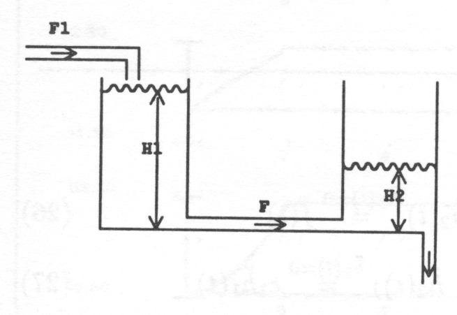
The system in Fig. 28 is used as an example of the difficulties caused by the lack of implicit knowledge on higher order derivatives.
| (23) | |||||
| (24) | |||||
| (25) |
The equations on the left carry the implicit information of the higher order derivatives. However, because the ISIR-algorithm cannot make full use of that implicit knowledge, the equations on the right are also included into the specifications to introduce explicitly the first order derivatives. In other words higher-order derivatives of state variables are included into the system state vector; see section 4.3.1. But when for example the signs of the first order derivatives do not tell whether is positive, negative or zero. To avoid this ambiguity, the third order derivative must be solved at points where .
| (26) | |||||
| (27) |
sys_eq([c(c1,C1),c(c2,C2),cv(h1,H1,D_H1),cv(h2,H2,D_H2),
        cv(f,F,D_F),cv(f1,F1,D_F1),cv(d_h1,D_H1,DD_H1),
        cv(d_h2,D_H2,DD_H2)],
        [_,_,_,_,_,_,DD_H2,DD_H1],[]):-
    F1 = 5,            D_F1 = 0,
    F = C1*(H1 - H2),  D_F = C1*(D_H1 - D_H2),
    D_H1 = F1 - F,     DD_H1 = D_F1 - D_F,
    D_H2 = F - C2*H2,  DD_H2 = D_F - C2*D_H2.

/* sign(D3_H1) = sign(DD_H2), sign(D3_H2) = sign(DD_H1) ! */

init(1,[c(c1,i(0.2,0.3)),c(c2,i(0.1,0.2)),cv(h1,p(0),_),
     cv(h2,p(0),_),cv(f,_,_), cv(f1,p(5),_),cv(d_h1,_,_),
      cv(d_h2,_,_)]).
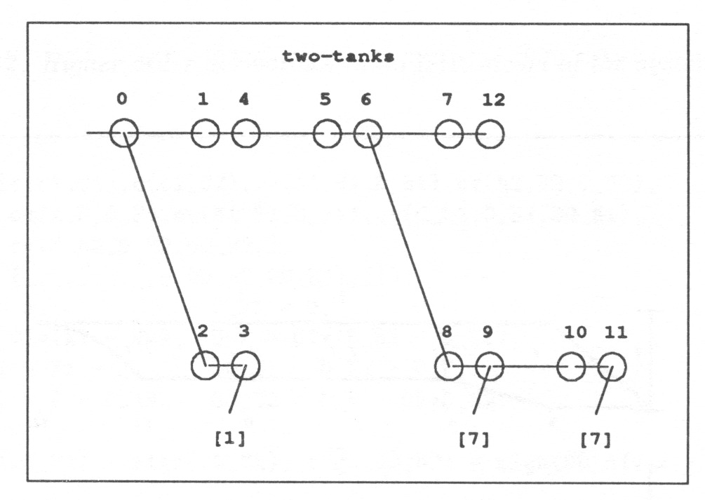
The list of the second order derivatives is added as an additional argument into the sys_eq-predicate in Table 32. Because only the sign of the second order derivative is needed at the points where the first-order derivative vanishes, it is not necessary to derive the exact value of the second-order derivative.
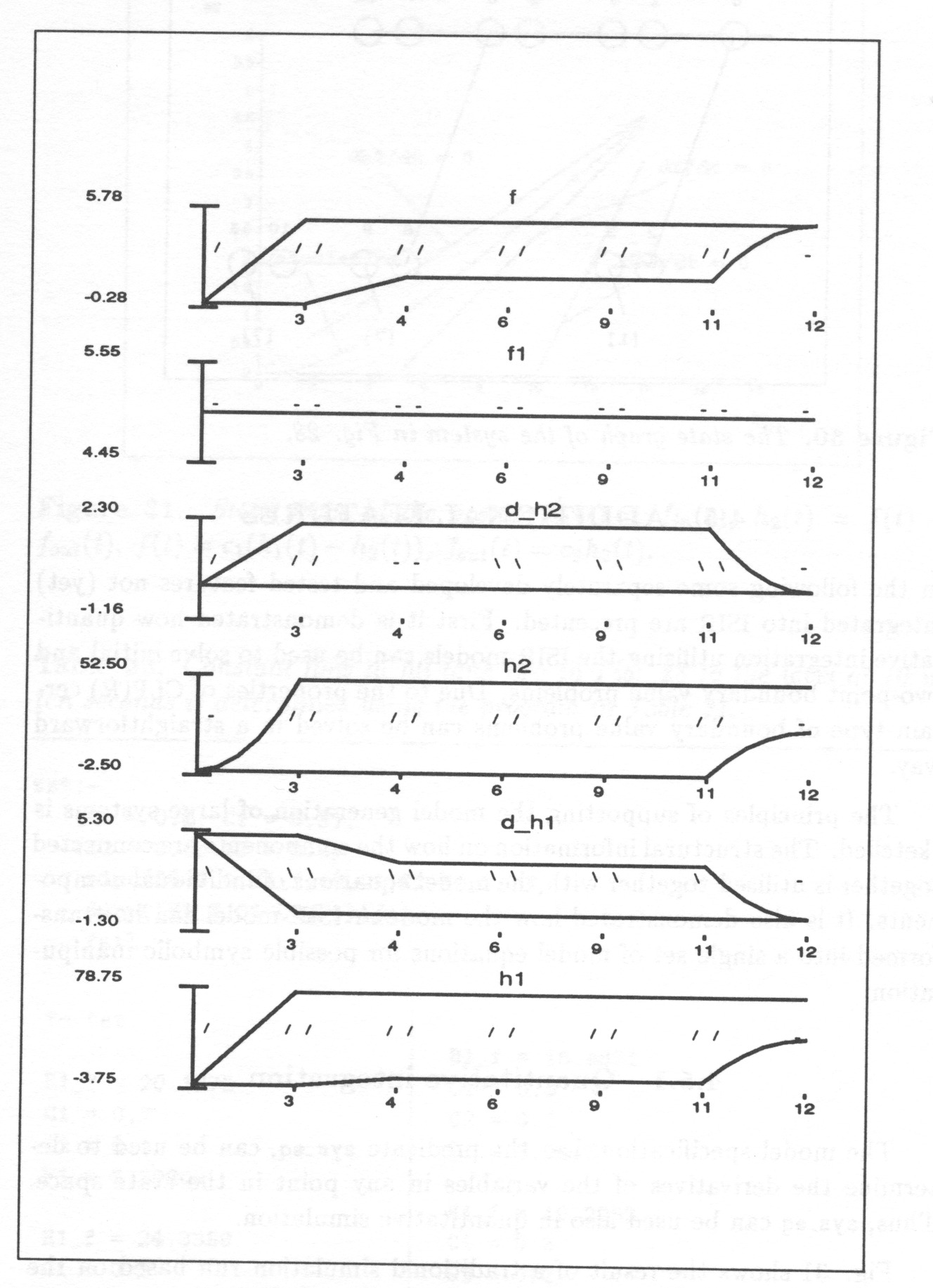
4.5 ADDITIONAL FEATURES
In the following some separately developed and tested features not (yet) integrated into ISIR are presented. First it is demonstrated how quantitative integration utilising the ISIR-models can be used to solve initial and two-point boundary value problems. Due to the properties of CLP() certain type of boundary value problems can be solved in a straightforward way.
The principles of supporting the model generation of large systems is sketched. The structural information on how the components are connected together is utilised together with the model equations of individual components. It is also demonstrated how the modular ISIR-model can be transformed into a single set of model equations for possible symbolic manipulation.
4.5.1 Quantitative integration
The model specification, i.e. the predicate sys_eq, can be used to determine the derivatives of the variables in any point in the state space. Thus,it can be used also in quantitative simulation.
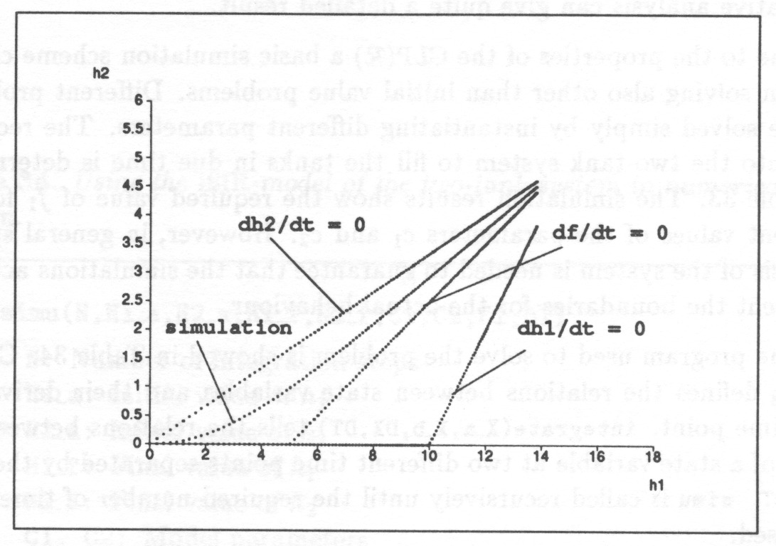
Fig. 31 shows the result of a traditional simulation run based on the specification in Table 32. The curve ‘simulation’ is a plot of a step response where the input has been changed from zero to one. It illustrates how clever discretization of the state space using some auxiliary variables results in quite a detailed partitioning of the state space. Hence, in principle qualitative analysis can give quite a detailed result.
Due to the properties of the CLP() a basic simulation scheme can be used in solving also other than initial value problems. Different problems can be solved simply by instantiating different parameters.
tst:-
   (C1 = 0.2; C1 = 0.3),
   (C2 = 0.1; C2 = 0.2),
    simu(50,0,0,H1_f,10,C1,C2,F1,0.2),
    dump([H1_f,C1,C2,F1]),nl,
    fail.
?- tst. H1_f = 20.1875 C1 = 0.2 C2 = 0.1 F1 = 3.39209 H1_f = 24.3358 C1 = 0.2 C2 = 0.2 F1 = 4.28548 |
H1_f = 16.4631 C1 = 0.3 C2 = 0.1 F1 = 3.04971 H1_f = 19.2252 C1 = 0.3 C2 = 0.2 F1 = 3.83392 |
The required flow into the two-tank system to fill the tanks in due time is determined in Table 33. The simulation results show the required value of for the different values of the parameters and . However, in general special analysis of the system is needed to guarantee that the simulations actually represent the boundaries for the actual behaviour.
The program used to solve the problem is showed in Table 34. Calling sys_eq defines the relations between state variables and their derivatives in a time point. integrate(X_a,X_b,DX,DT) tells the relations between the value of a state variable at two different time points separated by the time step DT. simu is called recursively until the required number of time steps is passed.
simu(N,H1_a,H2_a,H1_f,H2_f,C1,C2,F1,DT)
- N:
Number of integration steps
- H1_a:
Initial value of
- H2_a:
Initial value of
- H1_f:
Final value of
- H2_f:
Final value of
- C1, C2:
Model parameters
- F1:
Inflow into the system
- DT:
Integration time step
simu(N,H1_a,H2_a,H1_f,H2_f,C1,C2,F1,DT):-
   sys_eq([c(c1,C1),c(c2,C2),cv(h1,H1_a,D_H1),cv(h2,H2_a,D_H2),
         cv(f1,F1,_),cv(f,_,_),cv(d_h1,_,_),cv(d_h2,_,_)],_,[]),
   integrate(H1_a,H1_b,D_H1,DT),
   integrate(H2_a,H2_b,D_H2,DT),
   (N > 0
    -> simu(N-1,H1_b,H2_b,H1_f,H2_f,C1,C2,F1,DT)
     ; (H1_b = H1_f, H2_b = H2_f)).

integrate(Xa,Xb,Dx,Dt):-
   Xb - Xa = Dx*Dt.   there are more elegant algorithms

sys_eq([c(c1,C1),c(c2,C2),cv(h1,H1,D_H1),cv(h2,H2,D_H2),
        cv(f1,F1,D_F1),cv(f,F,D_F),cv(d_h1,D_H1,DD_H1),
        cv(d_h2,D_H2,DD_H2)],_,[]):-
   F = C1*(H1 - H2),
   D_F = C1*(D_H1 - D_H2),
   D_H1 = F1 - F,
   DD_H1 = D_F1 - D_F,
   D_H2 = F - C2*H2,
   DD_H2 = D_F - C2*D_H2.
Sometimes it is necessary to run a simulation which satisfies given, often quite rough, requirements. Something is typically required of the final state reached, and there are often some requirements on the way to reaching the final state. The above problem is simple and could be solved directly by a simple simulation run with CLP(), but in general this is not the case.
Fig. 32 shows a mass-spring system whose phase portrait is presented in Fig. 10 in the case where the control u is zero.
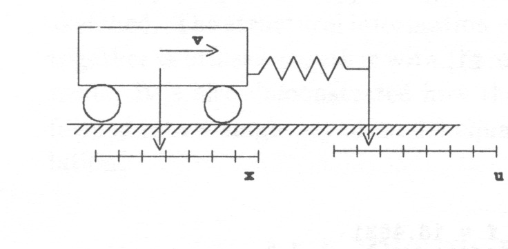
Let us assume that the carriage is initially standing still at and it must be moved to the position . Because there are infinitely many solutions to this problem, it is necessary to have some additional constraints. Typically, considering the time or the energy or the fuel spent is important. There may also be some strict limits on the controls or on the state. As a compromise between the real life problem and the complexity of its solution the sum of the time integral of the square of the force and the elapsed time multiplied by the constant is chosen as the criterium to be minimised.
| (28) | |||||
| (29) | |||||
| (30) | |||||
| (31) |
Applying variational calculus on the problem results in two additional differential equations of variables and and an equation from which optimal control can be resolved at any time point. In Table 35 the equations are given using the ISIR input formalism2222It is also possible to separate the actual system equations from the equations needed in solving the optimal control..
sys_eq(_,[c(k,K), u(u,U), cv(x,X,DX), cv(v,V,DV),cv(p1,P1,DP1),
        cv(p2,P2,DP2),c(h,H)],[]):-
       DX = V,
       DV = K*(U-X),
       DP1 = U-X+P2*K,
       DP2 = -P1,
       U-X+P2*K = 0,
      C + (U-X)*(U-X)/2 + P1*V + P2*K*(U-X) = H.
The problem is a typical two-point boundary value problem for which some of the boundary conditions are known at the initial time and the others at the final time. There are procedures in standard mathematical libraries to solve this kind of problems iteratively. However, it is possible to use CLP() to solve a class of two-point boundary value problems so that no iteration is needed for fixed final time problems. It is sufficient to ‘simulate’ the differential equations once from initial to final time using for example the integration scheme in Table 36 for each integration step.
sim(N,DT,[X0|[X1|XX]],Xf):-
   integrate(X0,X1,DT),
   sys_eq(_,X1,_),
    (N = 0 -> (XX = [], Xf = X1)
            ; sim(N-1,DT,[X1|XX],Xf)).

integrate([],[],_).
integrate([H0|T0],[H1|T1],DT):-
    integ(H0,H1,DT),
    integrate(T0,T1,DT).

integ(c(Id,X),c(Id,X),_).
integ(u(Id,_), u(Id,_),_).
integ(cv(Id,X,DX), cv(Id,X1,DX1),DT):- X1-X = (DX+DX1)/2*DT.
Because at the initial time not enough boundary conditions are known to determine constants of integration, the result of the ‘simulation’ is a large underdetermined set of equations. However, when the ‘simulation’ reaches the final time more boundary values are determined and the whole set of equations can be solved.
In the current example also the final time must be solved which complicates the solution procedure. Table 37 shows one of the alternative ways to solve the problem. The iterative simulation scheme is first executed for a given number of steps but having the integration time step uninstantiated ( sim(N_iter, DT, [X0|XX], Xf), !). After that instantiation is made ( goal(Xf, F, DF_DT). Newton iteration ( once(init_newt(0.2, DT, F, DF_DT), F = 0)) is applied to determine the integration time step DT so that the remaining boundary condition is satisfied resulting in the optimal trajectory shown in Fig. 33.
tpbv(N_iter,C):-
   retractall(newt(_,_,_)),
   sys_eq(_,X0,_),
   init(X0,C),
   sim(N_iter,DT,[X0|XX],Xf),!,
   goal(Xf,F,DF_DT),
   once(init_newt(0.2,DT,F,DF_DT), F = 0),
   tell('tpbv.dat'),
   outpt(0,DT,[X0|XX]),told.

goal([c(k,K),u(u,U),cv(x,1,DX),cv(v,0,DV),cv(p1,P1,DP1),
   cv(p2,P2,DP2),c(h,H), c(c,_)],H,1).
Newton iteration is implemented using assert and retract to allow iteration on backtracking as shown in Table 38. Another approach without backtracking is employed for example on page 50.
init_newt(X,X,E,DE_DX):-
    once(retractall(newt(_,_,_))),
    assert(newt(X,E,DE_DX)).
init_newt(_,X,E,DE_DX):- newt_iter(X,E,DE_DX).

newt_iter(X,E,DE_DX):-
    retract(newt(X0,E0,DE_DX0)),
    E0 + DE_DX0*(X1-X0) = 0,
    X = max(X0/2,min(2*X0,X1)),   % not too far in one step !
    printf('e: %  x: %  de_dx: %\n',[E0,X0,DE_DX0]),
    assert(newt(X,E,DE_DX)).
newt_iter(X,E,DE_DX):- newt_iter(X,E,DE_DX).
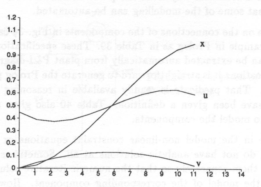
There are many design and analysis tasks which require solving control problems. The requirements are often quite vague. Sometimes discrete-event type control strategy is appropriate, but sometimes more sophisticated continuous time solution is needed. The above shows that the same model can be used for both purposes2323It might be possible to use the additional equations implied by the optimality principle also in the actual ISIR-algorithm to constrain the behaviours. However, this possibility has not yet been evaluated..
Consistent state transitions can also be determined by solving a set of two-point boundary value problems because the possible episodes are specified via the values of state variables and their derivatives at the end points of the episode. How to do this is demonstrated in section 7.
4.5.2 Support for the modelling of large systems
In the above examples the system specifications are written manually. However, the structure of the specifications is such that most of them can be generated automatically from process plant design documents. Automatic or at least semi-automatic computer-aided generation of the specifications is necessary in practice because the systems are large and complex.
The knowledge required in constructing the plant model can be grouped into:
-
Structural knowledge on how components are connected together. Such knowledge can be obtained from P&I-diagrams and other corresponding documents.
-
Operational characteristics of the components typically approximated with mathematical equations.
-
Knowledge on the laws of physics — like mass and heat balances — governing the phenomena taking place in the plant.
Part of the above knowledge can be conveniently presented as mathematical (differential) equations and inequalities, while some of the information is best represented using logic clauses.
When modelling large systems, the model should be generated systematically and in a tractable way from the plant documentation. The following shows that some of the modelling can be automated.
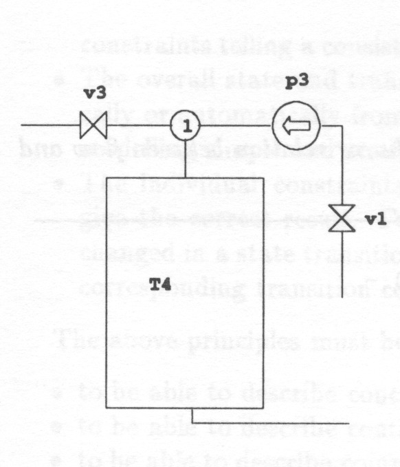
connected(valve(v1),pump(p3)).
connected(pump(p3),node(1)).
connected(valve(v3),node(1)).
 ...
connected(node(1),tank(t4)).
sys([V1,V3,P3,T4]):-
     valve(V1_in,V1_out,V1),
     pump(V1_out,P3_out,P3),
     valve(V3_in,V3_out,V3),
     tank(T4_in,T4_out,T4),
     sum([P3_out,V3_out,T4_in],0).

tank(Fin, Fout, M, Dm):- Dm = Fin - Fout.
%  h(P,V,M) = 0 if taking pressure into account

valve(0, 0, closed).
valve(F, F, open).
% valve(F, F, Pin, Pout,S):-   F = g(S)*sqrt(Pin - Pout).
The knowledge on the connections of the components in Fig. 34 can be represented for example in Prolog as in Table 39.
These specifications of the connections can be extracted automatically from plant P&I-diagrams. From these specifications it is straightforward to generate the Prolog predicate in Table 40. That predicate is readily available in reasoning after the components have been given a definition. Table 40 also gives some alternative ways to model the components.
There may be in the model non-linear constraint equations or even constraints which do not have analytic solutions at all. Sometimes it is sufficient to solve them separately so that the numeric iterative solutions are coded inside the model of the corresponding component. However, in general this is not the case but there are constraints which represent relations extending over many components2424It is very important to realize that although it is possible to make a modular description of the plant the resulting model may still be a set of equations which must be solved simultaneously.. Let us modify the earlier example on a network of valves to see how such relations can be handled, see Table 41. The model is constructed from components (‘modules’ or ‘objects’) connected together but the resulting model is still one set of simultaneous equations. CLP() prints out the equations when the model is called with all the arguments uninstantiated as shown in Table 42.
net(P1,P2,P3,P,F1,F2,F3,F4,s(0.1,0.3,0.6,1).
2 ?- net(P1,P2,P3,P,F1,F2,F3,F4,V1,V2,V3,V4).

V4 = open
V3 = open
V2 = open
V1 = open
F1 = F4 + F3 + F2
F4 = pow(P, 0.5)
1.66667*F3 = pow(-P3 + P, 0.5)
3.33333*F2 = pow(-P2 + P, 0.5)
10*F4 + 10*F3 + 10*F2 = pow(P1 - P, 0.5)
Other alternatives are given for other combinations for the valve states, but the above alone shows that in this case it is sufficient to provide the non-linear relations separate solutions, i.e. it is sufficient to code the solution inside the valve-predicate.
It can be concluded that CLP() allows modular modelling of the plant without forcing to try modular or object-oriented problem solving.
The main principles followed in the ISIR approach when modelling any industrial process can be summarised as follows:
-
A set of variables is selected to represent the state of the system. Typically the state variables represent the states of the components.
-
Some significant values of continuous time variables are marked as landmarks.
-
System time is considered as a sequence of time points and time intervals.
-
State transitions are modeled as transition constraints telling which pairs of old and new values of the variables are possible.
-
Mutual dependencies between state variables are modelled as state constraints telling a consistent system state from an inconsistent one.
-
The overall state and transition constraints are collected systematically or automatically from small individual constraints to make the modelling simple and straightforward.
-
The individual constraints must be complete so that they always give the correct result. For example, if a variable can remain unchanged in a state transition this alternative must be included in the corresponding transition constraint.
The above principles must be followed
-
to be able to describe concurrent phenomena;
-
to be able to describe continuous change;
-
to be able to describe complex dependencies between system components;
-
to avoid complex reasoning while modelling the system;
-
to allow a modular systematic approach to knowledge representation.
4.5.3 Support for the modelling of automatics
The goal of the research on the ISIR-algorithm is to develop a method for making use of deep knowledge of continuous time industrial processes in the design and V&V of discrete-event control strategies. The main difficulty is the representation of the knowledge of continuous processes and the reasoning based on it. Purely discrete dynamic systems are discussed a lot in the literature and there are tools and methods that can be applied if the basic ones already presented in this report are not sufficient. Thus, not much effort is put into this area, but the very principles of modelling the automatics in a way compatible with the ISIR-approach are discussed briefly.
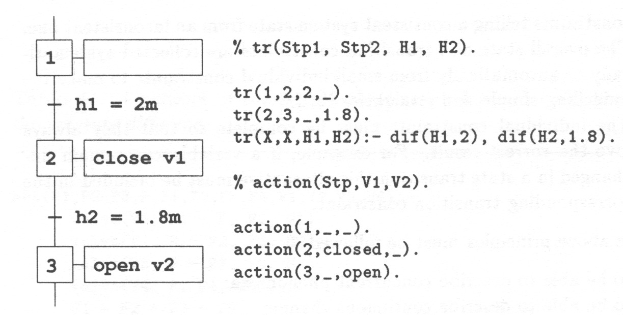
% tr(Stp1, Stp2, H1, H2).

tr(1,2,2,_).
tr(2,3,_,1.8).
tr(X,X,H1,H2):- dif(H1,2), dif(H2,1.8).

% action(Stp,V1,V2).

action(1,_,_).
action(2,closed,_).
action(3,_,open).
Control sequences with branches are best modelled as a hierarchy of sequences. On the top level an extra state vector is used to tell which of the low-level sequences are active and which are not.
Any non-branching sequence can be modelled according to the example in Fig. 35. tr specifies the possible transitions of the sequence, action constrains the possible values of an actuator.
The action-predicate does not tell for example what the value of v2 is in a state where Stp = 2. In such cases there are two alternatives:
-
•
Assume that in such a state v2 can be anything.
-
•
When considering automatics it can be assumed that the actuators change state only when explicitly told to. Thus, it can be assumed that if no command is given for an actuator, its state is preserved in the transition.
4.6 CHARACTERISTICS OF THE ISIR-ALGORITHM
In the following the ISIR-algorithm is related to some frequently discussed topics of qualitative reasoning.
Causality is often discussed in the context of model-based reasoning. In process plants the causality relations are often bi-directional, only control inputs and measurements have uni-directional causality relations towards the plant. In ISIR causality is not considered explicitly. For example the equation for the voltage and the current through a resistor is simply considered a constraint. In a typical case is marked constant to express the fact that and will change according to the external influence, but will not. But it is also possible to mark constant and let change if that choice reflects the system to be modelled.
Because in the ISIR-approach modelling the plant behaviour and modelling the control strategy are separated, uni-directional causality of control inputs can be modelled. When determining the plant state satisfying all the constraints related to a transition of the type the control inputs are considered constant. Correspondingly, when determining control inputs and control actions at a transition of type , the state variables can be considered fixed and only their derivatives may be assumed to change.
In this report applying model-based reasoning directly on on-line automatic control is not discussed. ISIR has many of the features needed for on-line control, but on-line control states also additional requirements not considered in the development of the ISIR-algorithm.
Correct abstraction level is emphasized in the literature. Models and problem solving tools should concentrate on those features of the system behaviour essential in solving the problems. In the context of discrete-event control such features are logic conditions, episodes during which some process variables are increasing or decreasing, and events at which something significant occurs. These are on the abstraction level used in ISIR.
In the following ISIR is related to ten requirements for a theory of change as presented by Shoham in [49]: A temporal language
-
•
should support statements that refer to time intervals;
In ISIR the system behaviour is considered as a sequence of time intervals separated by time points.
-
•
should allow representation of continuous change;
Representing continuous change is the main objective of the work on the ISIR-algorithm.
-
•
should avoid inter-frame problem ( It should not be necessary to list all the facts which are not changed by an action);
The consequences of an action are not listed explicitly. All the consequences not excluded by any of the given constraints are considered possible.
-
•
must allow representation of concurrent actions;
Concurrent behaviour does not need any specific representation. Concurrency is inherent in the ISIR-algorithm.
-
•
should avoid the intra-frame problem (Intra-frame problem: the result of an action depends also on other actions performed at the same time, not only on conditions prevailing when the action is initiated.);
Because the consequences of an action are not specified explicitly but via the constraints this problem is not encountered.
-
•
should allow representation of suppressed causation: natural death and delayed effect (Should allow modelling empirical associations of causal processes, not the actual causal processes in full detail);
This property is not yet included. However, some kind of a ‘qualitative timer’ included into the system state could be a solution. Its internal state and its output would be false until its input is triggered. Then its internal state would change to true after which its output could either change to true or remain false till a later time instant.
-
•
should allow representation of possible worlds (for example alternative future system states when action is either taken or not);
ISIR generates a state graph to represent the possible alternative futures.
-
•
should avoid cross-world identification problem (should allow selective identification of propositional tokens in two possible worlds);
The only significant tokens in different system states are the values of system state variables which can be easily identified.
-
•
should allow easy modification of knowledge, (modularity);
It is possible to make the modification of the knowledge easy. Currently the knowledge must be provided as logic clauses and mathematical equations, which is sufficient for small systems.
-
•
should have a computational framework.
The ISIR-algorithm is the computational framework.
That ISIRsatisfies the above requirements does not prove that it implements a general theory of change. However, it indicates that on its restricted domain it satisfies the basic requirements.
5 A POWER PLANT FEEDWATER SYSTEM
Work done elsewhere has demonstrated the suitability of Prolog in solving problems of logic. Being a ‘dialect’ of Prolog CLP() provides the same power of solving logic ‘puzzles’. The examples in the previous chapters have shown that ISIR supports the integration of discrete and continuous domains. They have also shown the soundness of the principles in dealing with the continuous systems.
A power plant feedwater system is modelled and analyzed in the following to test ISIR with a more realistic system. To work with a real life example it is necessary to have tools which support the generation of the ISIR model. Because such a tool does not yet exist, a simplified feedwater system is analyzed. In spite of the simplification the model is much more complex than those in the previous examples. In addition it demonstrates how to deal with some aspects of systems not encountered when working with the proof-of-the-principle cases. For example there are constraints which do not have analytic solutions. The example shows how numerical iteration can be applied to deal with such constraints.
ISIR requires that the system model is a constraint which can be used to solve any of the variables as a function of the others. The low-level piece of knowledge needed is a ‘Prolog-style’ relation between system state variables.
Much of the plant operation is based on taking discrete control actions. Control sequences are based on reasoning like
“When I take action a, will start to increase. When I will take actions b and c so that …”
“All the time I have to worry about not getting too high and …”
“Pumps and valves have all kinds of restrictions of operation which I have to remember.”
“The other parts of automatics may have some effect on the part I am now designing”
In the design and verification of plant automatics it is important to know the relationships between process variables. Often the only available but fortunately also sufficient knowledge for early design phases is abstract qualitative knowledge. For automated reasoning such knowledge is also most appropriate. However, for example the properties of saturated steam are difficult to describe qualitatively. Fortunately there is no reason to do that because there is accurate knowledge on the properties of the saturated steam and because it is possible to make efficient use of appropriately presented quantitative knowledge in automated reasoning.
5.1 HEAT EXCHANGERS
Heat exchangers and the steam generators are central components of a feedwater system. Two phenomena must be modelled to handle them properly: properties of saturated steam and water, and heat transfer through the heat exchanger wall.
The properties of saturated steam and water were first tried to be approximated with low order polynomials allowing analytic solution, documented as alternative B later in this section. However, the result was not satisfactory and higher order polynomials were chosen and iterative solutions of the problems were employed. This approach was easy to implement and gave good enough results. It should also be possible to use existing codes for the properties of steam and water to get more accurate results. However, integrating them into the ISIR-algorithm requires some C- and unix-programming which might be laborious and is thus left for ‘some later time’.
5.1.1 Saturated steam in a drum
The underlying thermodynamics of this section are presented for example in [1].
The system equations
Fig. 36 shows a tank filled with saturated steam and water in thermodynamic balance. Water is pumped into the tank (). Saturated steam can be let out of the drum (). Heat is flowing into the drum ().
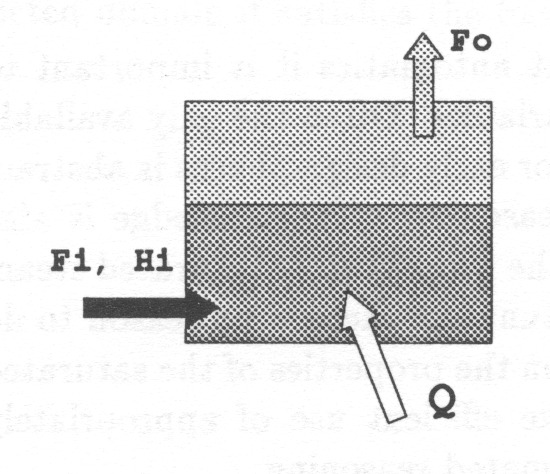
The system obeys the following equations:
| (32) | |||||
| (33) | |||||
| (34) | |||||
| (35) | |||||
| (36) | |||||
| (37) | |||||
| (38) | |||||
| (39) |
where
Approximative equations for steam properties, A
The thermodynamic state of the system can be described by any two of the state variables where is the specific volume, the specific enthalpy, the temperature and the steam content of the thermodynamic system. can be replaced by pressure because it is a function of . As the equations 32 – 39 show, a definition for a general relation is necessary. It should tell the values of the other state variables when any two of them are known. Because control aims in changing the system state, it is necessary to consider also the rates of change so that actually to determine a relation must be determined.
The equations
| (40) | |||||
| (41) |
where
-
:
specific volume of the mixture of steam and water
-
:
specific volume of saturated water
-
:
specific volume of saturated steam
-
:
specific enthalpy of the mixture of steam and water
-
:
specific enthalpy of saturated water
-
:
specific enthalpy of saturated steam
-
:
proportion of steam in the mixture of steam and water
-
:
temperature of the mixture of steam and water
tell the relations between and . are tabulated as functions of (or ). Also the relation between and is tabulated.
The functions can be approximated successfully with low order polynomials of temperature2525T can be replaced with p or any function of either p or T, for example . T. Here the approximating polynomials are determined by minimising the following weighed square error
| (42) |
From an equation , CLP() can directly solve if and are known or it can solve if and are known. But because CLP() cannot solve directly even if and are known must be given an explicit solution as a function of and .
To provide a general constraint representing the equations 40 and 41 they, and the solution of from them, must be represented as a CLP()-constraint. If is known CLP() can directly solve and . A CLP()-predicate is constructed which waits until and and or and are known and if is not yet known it is solved with Newton iteration:
| (43) |
For example, for solving from and , the iteration is implemented as shown in Table 43.
newt_stvh(N, V, H, X, T, Tf):-
   N >= 0,
   hv(Hw,DHw,Hs,DHs,Vw,DVw,Vs,DVs,T),
   Xa = (V - Vw)/(Vs - Vw),
   DX = (-DVw*(Vs - Vw) - (V-Vw)*(DVs-DVw))/(Vs-Vw)/(Vs-Vw),
   F = Hw + Xa*(Hs - Hw) - H,
   DF = DHw + Xa*(DHs - DHw) + DX*(Hs-Hw),
   F + DF*(T1-T) = 0,
   (N*1e4*F = 0
       -> (T1 = Tf, T1 = T, X = Xa)
       ; (T1 > 0, T1 < 400, newt_stvh(N-1, V, H, X, T1, Tf))),!.

% relations between steam parameters

hv(Hw0,D_Hw0,Hs0,D_Hs0,Vw0,D_Vw0,Vs0,D_Vs0,T0):-
        % some scaling
         T = (T0 + #abs_zero)/100,
         Vw = 1000*Vw0,       D_Vw = 1e5*D_Vw0,
         10*Vs = 1/Vs0,       1000*D_Vs0 = -D_Vs/Vs/Vs,
         Hw = Hw0/100,        D_Hw = D_Hw0,
         Hs = Hs0/1000,       D_Hs = D_Hs0/10,
         % interpolation
         f3(Hw, D_Hw, T, #ahw, #bhw, #chw, #dhw),
         f3(Hs, D_Hs, T, #ahs, #bhs, #chs, #dhs),
         f3(Vw, D_Vw, T, #avw, #bvw, #cvw, #dvw),
         f3(Vs, D_Vs, T, #avs, #bvs, #cvs, #dvs).

f3(F,DF,X,A,B,C,D):-
         F = A*X*X*X + B*X*X + C*X + D,
         DF = 3*A*X*X + 2*B*X + C.
The predicate newt_stvh is called only when remains unknown (= is not ground after all the variables to be instantiated are already instantiated2626The meta-logical features of CLP() make it easy to control the computation according to which variables have not yet been solved. Note that when programming a general-purpose predicate it cannot be anticipated which of the variables, if any, are known and which are not.). Thus the problem solving capabilities of CLP() are not needed in this case and the iteration could as well be implemented in for example the programming language C. In this way efficient existing numerical routines could be applied.
The resulting constraint was tested on a pressure range from 3.5bar to 60bar for x-values 0, 0.05, 0.5, 0.95 and 1. In the test, all the possible pairs of were chosen as base variables to solve the other two. There were altogether 735 test cases. In 733 cases all the prediction errors where less than 2%. In the remaining two cases the constraints failed altogether. This occurred because the maximum value of in the test data is 2802.3 and the maximum of the estimate of obtained by 42 is slightly less than that.
Because the ISIR-algorithm searches for minima and maxima of state variables, points where gradients vanish must be solved as well. For saturated steam, when x is high enough and for a narrow region . The extremes can be solved analytically when are approximated with third order polynomials of T. In the general case the extremes must be searched iteratively. Table 44 shows how to solve the maximum of when is known.
hill_stxh(N, X, H, V, T, Tf):-
   N >= 0,
   hv(Hw,DHw,Hs,DHs,Vw,_,Vs,_,T),
   hv(Hw1,DHw1,Hs1,DHs1,Vw1,_,Vs1,_,T+1),
   DF = DHw + X*(DHs - DHw),
   DF1 = DHw1 + X*(DHs1 - DHw1),
   DF + (DF1-DF)*(T1-T) = 0,
   (T1 = T
    -> (T1 = Tf, V = Vw + X*(Vs-Vw), Hw + X*(Hs-Hw) = H)
    ; (T1 > 0, T1 < 400, hill_stxh(N-1,X,H,V,T1,Tf))),!.
Note that the second order derivatives are not solved analytically but differences are used instead.
Summary
A CLP() predicate, fully compatible with the CLP() problem solving, is constructed to tell the relation between the properties of the saturated steam. This allows reasoning on the behaviour of various systems containing saturated steam.
Approximative equations for steam properties, B
Trying to solve equations 40 and 41 analytically gives 4th order polynomials even when using 2nd order interpolating polynomials. The equations can be rewritten so that it is sufficient to solve equations of the degree no higher than the interpolating polynomials allowing analytic solution instead of numeric iteration.
In a test the coefficients and were interpolated with second order polynomials of so that it was easy to code analytic solution for the equations. The resulting constraint was tested on a pressure range from 3.5bar to 60bar and for x-values 0, 0.05, 0.5, 0.95 and 1. In the test all the possible pairs of were chosen as base variables to solve the other two. There were altogether 733 test cases. In 49 cases the program did not succeed to pass the 5% error margin. Typically prediction failed at when predicting the other variables as a function of and or and and at or when predicting the other variables as a function of and .
The low accuracy is revealed in situations not encountered in typical examples. However, it is evident that if this approach is applied, at least third order polynomials should be used.
Examples
sys_eq([c(vvhex,VVhex), u(fohex,Fohex,_), u(fihex,Fihex,_),
    cv(xhex,Xhex,D_Xhex), cv(phex,Phex,D_Phex), u(q,Q,std)]
    ,_, [Frz2,Frz4,Frz5]):-
     st_drum(VVhex,Phex,D_Phex,_, _,Xhex,D_Xhex, Fihex-Fohex,
          Fihex*Hshex-Fohex*Hwhex - Q, Frz2),
     sat_steam(Phex,_, _,_,_,_,Hshex,_,1,_, Frz4),
     sat_steam(Phex,_, _,_,_,_,Hwhex,_,0,_, Frz5).

st_drum(VV,P,DP,T,DT,X,DX,DM,Q,Frz):-
     V*M = VV, DV*M + V*DM = 0,
     DH*M + H*DM = Q,
     sat_steam(P,DP,V,DV,T,DT,H,DH,X,DX,Frz).
id       magnitude    derivative  ->    magnitude    derivative
vvhex      100             -       =       100           -

fohex        5             ?       d         5           x
fihex        ?             ?       m         5           x
xhex      0.65             0       =      0.65           0

phex        20             0       =        20           0

q            ?            std      m      9444          std


id       magnitude    derivative  ->    magnitude   derivative
vvhex      100             -       =       100         -
fohex        ?             ?       m     5.294         x
fihex        ?             ?       m     5.294         x
xhex      0.65             0       =      0.65         0
phex        20             0       =        20         0
q        1e+04            std      =     1e+04        std

id       magnitude    derivative  ->    magnitude   derivative
vvhex      100             -       =       100          -
fohex        ?             ?       m        0|5.294     x
fihex        ?             ?       m   0.5232|5.294     x
xhex      0.65       -1e+05|0      d      0.65      -0.0022|0

phex        20             0       =        20          0
q        1000|1e+0        std      =     1000|1e+04    std

id       magnitude    derivative  ->    magnitude   derivative
vvhex      100             -       =       100         -
fohex       3|10           ?       d        3|10       x
fihex       3|10           ?       m    5.267|10       x
xhex      0.65       -1e+05|0      d      0.65     -0.00098|0

phex        20             0       =        20         0
q       1e+04|3e+0        std      m    1e+04|1.889e+04  std


id       magnitude    derivative  ->    magnitude   derivative
vvhex      100             -       =       100          -
fohex       5|10           ?       d        5|10        x
fihex        ?             ?       m        5|10        x
xhex       0.5             0       =       0.5          0
phex       10|20           0       =       10|20        0
q            ?            std      m   9444|2.014e+04  std
In Table 46 there are some test results of the program in Table 45 which implements the equations 32 – 39 in a case where saturated steam in the pressure of the drum is lead into it and saturated water is lead out of the drum. The columns on the left of `->' represent the a priori knowledge of the values of the variables. ‘?’ indicates that there are no constraints on the corresponding variable. ‘l|h’ indicates an interval from l to h.
5.1.2 Heat flow through a heat exchanger wall
The heat flow Q in Fig. 36 is established in the heat exchanger in Fig. 37 with water flowing in a pipe through the water section of the drum. In the following a simple approximative equation for the heat transfer is derived.
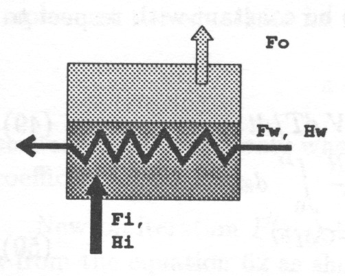
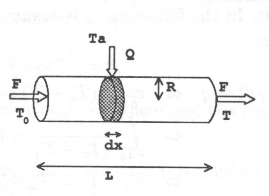
There is a constant flow F through the pipe. Let us consider a small slice of the mass flowing in the pipe and a small time interval so that
The area of the slice is and its volume is .
| (47) | |||||
| (48) |
The heat flowing into the slice is . The specific heat capacity at constant pressure is defined with the equation . In the following is assumed to be constant with respect to temperature.
| (49) | |||||
| (50) | |||||
| (51) |
5.2 A FEEDWATER SYSTEM
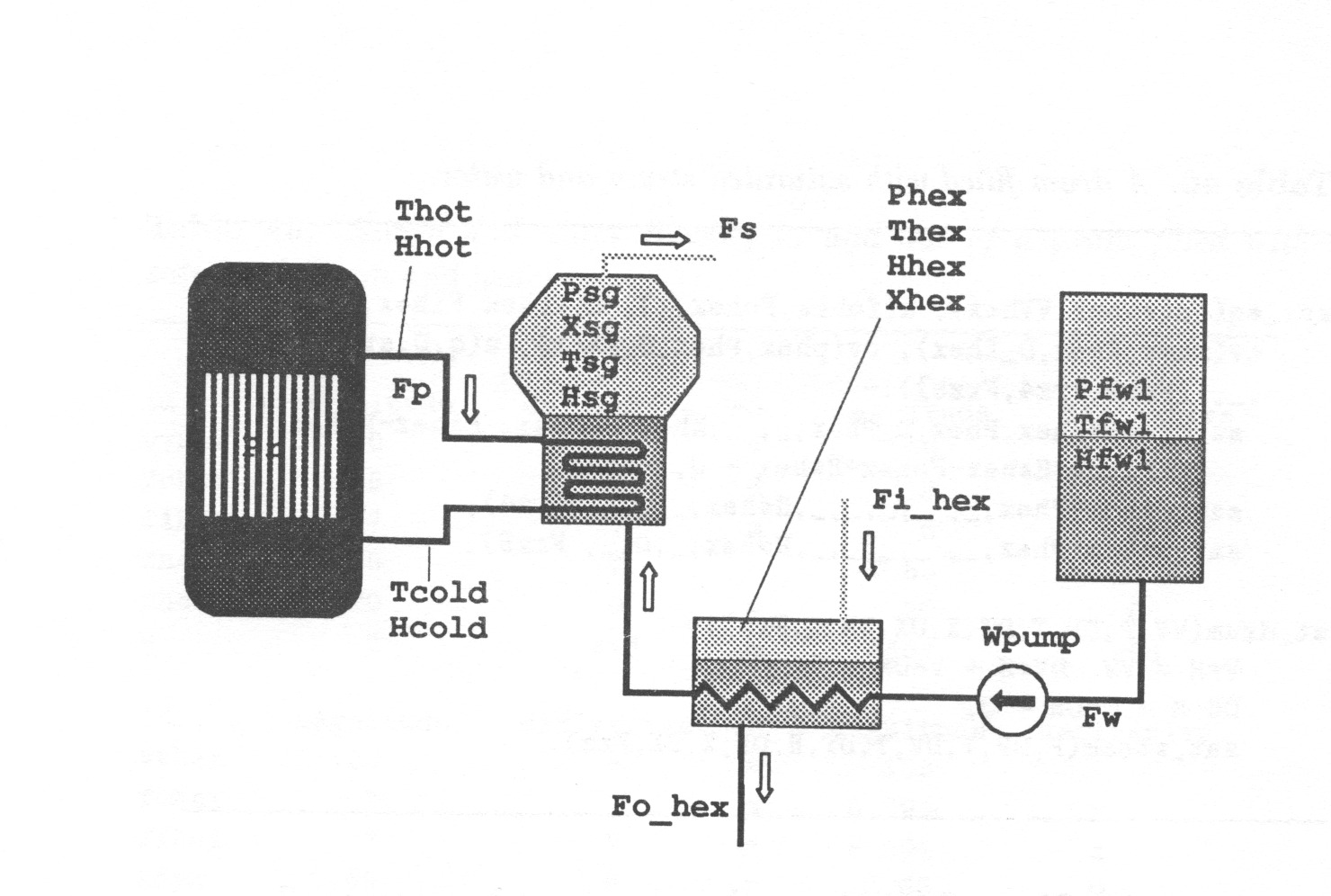
A model of the system in Fig. 39 is constructed and used to solve some low level problems related to reasoning on the system behaviour. Some of the model equations are rough approximations, because the purpose of the example is more to demonstrate the principles than to derive highly accurate representations on the modelled phenomena. The main program implements the following equations
| (52) | |||||
| (53) | |||||
| (54) | |||||
| (55) | |||||
| (56) | |||||
| (57) | |||||
| (58) | |||||
| (59) |
The model is a CLP() predicate sys_eq in Table 47 where sat_steam is a predicate telling the properties of saturated steam and st_drum is a constraint for a drum containing saturated steam. In the CLP() model the derivatives of the constraints are written explicitly.
sys_eq(Time,[Stp,c(khex,Khex), c(ksg,Ksg), c(vvhex,VVhex),
       c(vvsg,VVsg), c(mr,Mr), c(fp,Fp), cv(pfw1,Pfw1,D_Pfw1),
       cv(ffw,Ffw,D_Ffw), cv(fohex,Fohex,D_Foh),
       cv(fihex,Fihex,D_Fih),cv(xhex,Xhex,D_Xhex),
       cv(phex,Phex,D_Phex), cv(xsg,Xsg, D_Xsg),
       cv(psg,Psg,D_Psg), cv(thot,Thot, D_Thot), cv(fs,Fs,D_Fs),
       cv(pr,Pr,D_Pr)],Frz):-

    water(Thot,D_Thot,_,D_Hhot),
    Mr*D_Hhot = 1000*Pr - Qsg,
    D_Msg = Ffw - Fs,
    st_drum(VVsg,Psg,D_Psg,Tsg,_,Xsg,D_Xsg,D_Msg, Q, Frz1),
    st_drum(VVhex,Phex,D_Phex,Thex, _,Xhex,D_Xhex,Fihex-Fohex,
       Fihex*Hshex-Fohex*Hwhex - Qhex, Frz2),
    sat_steam(Psg, _, _,_,_,_,Hsteam,_,1,0, Frz3),
    sat_steam(Phex,_, _,_,_,_,Hshex,_,1,_, Frz4),
    sat_steam(Phex,_, _,_,_,_,Hwhex,_,0,_, Frz5),
    sat_steam(Pfw1,D_Pfw1,_,_,Tfw1,D_Tfw1,Hfw1,_,0,_, Frz6),
    water(Tpump-Tfw1, D_Tpump - D_Tfw1, Wpump, D_Wpump),
    Psg - Pfw1 = 1000*Wpump,
    D_Psg - D_Pfw1 = 1000*D_Wpump,
    Tsg_diff = 4.3*(Thot - Tsg),
    Q = Qhex + Ffw*(Hfw1+Wpump) + Qsg - Fs*Hsteam,
    Thex_diff = 4.3*(Thex-Tpump),
    conduct(-Qsg, Tsg_diff, -Tsg_diff, Ksg, Fp),

xexp(Qsg-Q+D_Msg*Hsteam,Hfw1+Wpump-Hsteam+Thex_diff,-Thex_diff,
         Khex,Ffw, Frz7).

st_drum(VV,P,DP,T,DT,X,DX,DM,Q,Frz):-
    V*M = VV, DV*M + V*DM = 0,
    DH*M + H*DM = Q,
    sat_steam(P,DP,V,DV,T,DT,H,DH,X,DX,Frz).

water(T,DT,H,DH):-
    H = 800 + 4.3*(T - 180),
    DH = 4.3*DT.
The variable stp has no meaning here. Such discrete variables can be used e.g. to designate the state of an automatic control sequence.
st_drum implements the equations
| (60) | |||||
| (61) |
st_drum specifies the properties of saturated steam and water implements a rough approximation of the specific enthalpy of water. conduct and xexp implement the equations for heat transfer.
| (62) |
conduct can be used only when the primary side flow and the heat transfer coefficient are known.
conduct(A,B,C,K,X):- A + B*X + C*X*pow(#e, -K/X) = 0.

xexp(A,B,C,K,X,Frz):-
    A + B*X + C*X*pow(#e, -K/X) = 0,
    Frz = freeze(l(A,B,C,K),xexp2(0,A,B,C,K,0.001,X)).

xexp2(N,A,B,C,K,X,Xf):-
    N < 20, X > 0,
    A + B*X + C*X*pow(#e, -K/X) = Y,
    DY = B + C*pow(#e, -K/X)*(1 + K/X),
    (Y = 0
         -> X = Xf
         ; (Y + DY*(X1 - X) = 0,
xexp2(N+1,A,B,C,K,X1,Xf))),!.
The example in Table 49 shows how system state can be determined when some of the variables are known. If for example had been given a positive value the result would show how to make increase. Another way to see what is needed to increase is to compare two plant states having different values of as the second example shows.
id magnitude deriv -> magnitude derivative stp 1 - = 1 - khex 600|1000 - = 600|1000 - ksg 6000|1e+04 - = 6000|1e+04 - vvhex 100 - = 100 - vvsg 1000 - = 1000 - mr 1e+04 - = 1e+04 - fp 5000 - = 5000 - pfw1 7 0 = 7 0 ffw ? 0 m 160 0 fohex ? 0 m 20.97|21.43 0 fihex ? 0 m 20.97|21.43 0 xhex 0.7 0 = 0.7 0 phex 22 0 = 22 0 xsg 0.5 0 = 0.5 0 psg 45 0 = 45 0 thot ? 0 m 273.3|277.2 0 fs 160 0 = 160 0 pr ? 0 m 296|296.9 0 id magnitude derivative -> magnitude derivative stp 1 - = 1 - khex 600|1000 - = 600|1000 - ksg 6000|1e+04 - = 6000|1e+04 - vvhex 100 - = 100 - vvsg 1000 - = 1000 - mr 1e+04 - = 1e+04 - fp 5000 - = 5000 - pfw1 7 0 = 7 0 ffw 160 0 m 320 0 fohex 20.97|21.43 0 m 36.36|41.06 0 fihex 20.97|21.43 0 m 36.36|41.06 0 xhex 0.7 0 = 0.7 0 phex 22 0 = 22 0 xsg 0.5 0 = 0.5 0 psg 45 0 = 45 0 thot 273.3|277.2 0 m 289.4|297.6 0 fs 160 0 m 320 0 pr 296|296.9 0 m 595.4|604.1 0
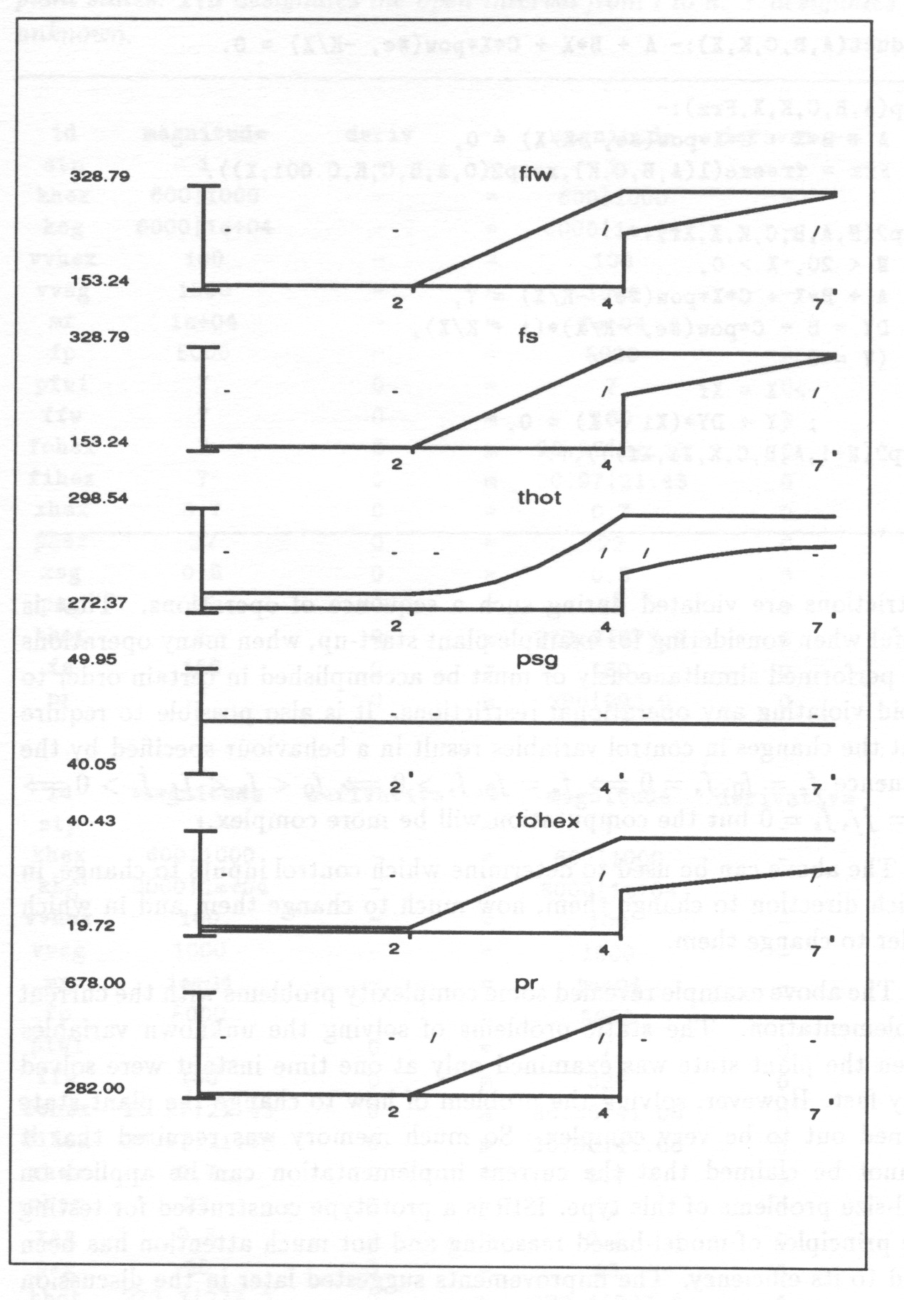
From the parameters whose value has changed above is the primary control variable2727 Nothing determines the derivatives of the control variables and they affect only derivatives of some other variables. Control variables can be identified automatically.. . The analysis can be made more detailed by checking what happens in the sequence . Fig. 40 show the results of such an analysis. In addition to producing such figures ISIR can check automatically whether any of the given operational restrictions are violated during such a sequence of operations. That is useful when considering for example plant start-up, when many operations are performed simultaneously or must be accomplished in certain order to avoid violating any operational restrictions.
It is also possible to require that the changes in control variables result in a behaviour specified by the sequence but the computation will be more complex.
The above can be used to determine which control inputs to change, in which direction to change them, how much to change them and in which order to change them.
5.3 Discussion
The above example revealed some complexity problems with the current implementation. The static problems of solving the unknown variables when the plant state was examined only at one time instant were solved very fast. However, solving the problem of how to change the plant state turned out to be very complex. So much memory was required that it cannot be claimed that the current implementation can be applied on real-size problems of this type. The complexity could be reduced with the following measures:
- General Optimization of the Code
-
In addition to employing the previously presented techniques no explicit attention is paid on the complexity of the program. Careful analysis of the code might reveal possibilities to reduce the complexity.
- Reorganising the Main Program
-
Especially the main program should be examined for optimisation. For example, in addition to inserting the new states in the state graph they are also unnecessarily stored for long times in temporary lists of states whose successors have not yet been identified.
- Optimizing the Determination of Consistent Transitions
-
The analysis of consistent transition is complex and frequently used thus having a great influence on the overall complexity of the program. The complexity is due to extra alternatives in a predicate which guarantees that a solution is found also in rare special cases. A more effective solution could make the program much faster. However, this is the central and most difficult part of the algorithm so that finding a better solution might require a lot of work.
- Using C for Numeric Iteration
-
Currently many numeric problems are solved with Newton iteration implemented recursively in CLP(), which is evidently an inefficient solution. In the next version of CLP() there may be a better interface to other languages so that existing efficient numeric routines can be employed.
- Constraining the Search Space
-
Requiring only that the plant must be moved into a given state results in a lot of trial-and-error search because the requirement constrains the search space poorly. This is because the plant system integrates the inputs many times so that the effect of a change in a control input in some of the state variables can be seen only at a later time. It is possible to constrain the search space with additional constraints, but it is difficult to generate such constraints automatically. Requiring the user to give such constraints may result in a situation where the user rather than the tool solves the problem.
- Employing Numeric Integration
-
The consistent transition can be determined with numeric integration if the task is considered as a two-point boundary value problem. Solving such problems requires a lot of iteration but if the requirement of proper handling of uncertain models is alleviated the results might be obtained fast enough. The approach requires some preparatory work which may be difficult to automate so that the manual work related to plant modelling increases.
ISIR is a prototype constructed for testing the principles of model-based reasoning and not much attention has been paid to its efficiency. The improvements suggested above would make it more efficient. However, solving control problems will always be complex and also the improved version of ISIR would require a lot of computing capacity.
6 A CONTINUOUS STIRRED TANK REACTOR
One important feature of a design tool is to detect such significant situations and characteristics of the system behaviour which may remain undetected in manual scrutiny. ISIR-models represent a class of real-life systems resulting in predictions representing a class of behaviours. Because qualitatively significantly different possible behaviours are presented as alternative classes of predictions they are easy to detect. The following is a test on how well the algorithm can distinguish relatively similar behaviours of a system having somewhat complicated dynamics.
The system to be analysed has three steady states. A minor change in the input may make the system drift from one steady state to another. Evidently this is a significant pattern of behaviour but at the same time it is a challenge for tools relying on rough plant models and qualitative methods.
The example demonstrates also the multiparameter Newton iteration.
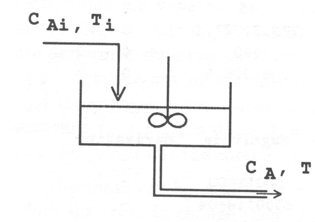
In [11] Dalle Molle analyzes with QSIM a continuous stirred tank reactor shown in Fig. 41. He presents the following model equations for an irreversible exothermic first-order reaction taking place in the reactor:
| (63) | |||
| (64) | |||
| (65) | |||
| (66) |
where
-
:
The concentration of A in the tank and in the exit stream
-
:
The concentration of A in the inlet stream
-
:
The temperature in the tank and in the exit stream
-
:
The temperature in the inlet stream
-
:
Residence time or space velocity (tank volume/inlet flow rate)
-
:
Rate of reaction of A
-
:
Reaction rate constant
-
:
The heat of reaction (divided by solution density and heat capacity)
-
:
The rate constant pre-exponential
-
:
activation energy (divided by the universal gas constant)
In Table 50 the above equations are written into the formalism required by the ISIR-algorithm.
sys_eq([dv(iter_mod,_),c(k0,K0),c(e,E),c(tau,Tau),c(h_diff,H_dif
f),
  c(ca_in,Ca_in), c(t_in,T_in),cv(t,T,D_T),cv(ca,Ca,D_Ca)],
   [_,_,_,_,_,_,_,D_Ca,-Ca*D_T],[]):-
    K0*pow(#e,-E/T)*Ca = Ra,
    D_Ca = (Ca_in - Ca)/Tau - Ra,
    D_T = (T_in - T)/Tau - H_diff*Ra.
It can be easily shown that has the same sign as the third-order derivative of and has the same sign as the third-order derivative of . Thus, they are used in the higher order derivative constraints.
After having instantiated some of the variables the ISIR-algorithm applies the predicate local_extrem to instantiate the possibly remaining uninstantiated variables. It can be used for example to determine e.g. the points where the derivatives of some of the variables vanish. Here the predicate local_extrem is used to determine the solution of the system equations in those cases where the CLP() internal equation solver cannot find the solution2828The same iterative solution could be implemented also inside the predicate sys_eq.
Newton iteration is applied to find the zeroes of the functions and . The iteration is started either from the point (alternative a) or from the point (alternative b). The derivatives of and needed in the iteration are approximated with differences by computing their values at three points. Table 51 shows how the iteration is implemented.
local_extrem([dv(iter_mod,Mode),c(k0,K0),c(e,E),c(tau,Tau),
    c(h_diff,H_diff),c(ca_in,Ca_in), c(t_in,T_in),cv(t,T,D_T),
    cv(ca,Ca,D_Ca)]):-
   ((T0 = 600, C0 = 0, Mode = a); (T0 = 340, C0 = 1, Mode = b)),
   iterate(30,[dv(iter_mod,Mode),c(k0,K0),c(e,E),c(tau,Tau),
   c(h_diff,H_diff), c(ca_in,Ca_in), c(t_in,T_in),cv(t,T0,D_T),
   cv(ca,C0,D_Ca)],T,Ca).

local_extrem(_).

iterate(N,[dv(iter_mod,Mode),c(k0,K0),c(e,E),c(tau,Tau),
   c(h_diff,H_diff),c(ca_in,Ca_in), c(t_in,T_in),cv(t,T0,D_T),
   cv(ca,Ca0,D_Ca)],Tf,Caf):-
  N > 0,
  sys_eq([dv(iter_mod,Mode),c(k0,K0),c(e,E),c(tau,Tau),

c(h_diff,H_diff),c(ca_in,Ca_in),c(t_in,T_in),cv(t,T0,D_T+Faa),
       cv(ca,Ca0,D_Ca+Gaa)],_,[]),
  ground([Faa,Gaa]),

  sys_eq([dv(iter_mod,Mode),c(k0,K0),c(e,E),c(tau,Tau),
          c(h_diff,H_diff),c(ca_in,Ca_in),c(t_in,T_in),
          cv(t,T0+1,D_T+Fba),cv(ca,Ca0,D_Ca+Gba)],_,[]),

   sys_eq([dv(iter_mod,Mode),c(k0,K0),c(e,E),c(tau,Tau),
           c(h_diff,H_diff),c(ca_in,Ca_in),c(t_in,T_in),
           cv(t,T0,D_T+Fab),cv(ca,Ca0+#eps,D_Ca+Gab)],_,[]),

   Faa + (Fba-Faa)*(T1-T0) + (Fab-Faa)*(Ca1-Ca0)/#eps = 0,
   Gaa + (Gba-Gaa)*(T1-T0) + (Gab-Gaa)*(Ca1-Ca0)/#eps = 0,

   (N*1000*(abs(Faa)+abs(Gaa)) = 0
     -> (T0 = Tf, Ca0 = Caf, Faa = 0, Gaa = 0)
     ;
iterate(N-1,[dv(iter_mod,Mode),c(k0,K0),c(e,E),c(tau,Tau),
               c(h_diff,H_diff),c(ca_in,Ca_in), c(t_in,T_in),
               cv(t,T1,D_T),cv(ca,Ca1,D_Ca)],Tf,Caf)), !.
The alternatives a and b often give different solutions. For example equations LABEL:eq:cstrc and LABEL:eq:cstrt have for certain parameter values three different steady state solutions, one of them captured by the alternative a, an other captured by the alternative b and the third one, an unstable steady state is not captured at all. Evidently a more sophisticated approach is needed to solve this type of problems. However, to demonstrate the results that can be obtained by making a distinction between multiple solutions of the system equations the above two alternatives are applied.
The model is tested by simulation starting from a steady state where as specified in Table 52. At some time during the simulation the concentration is reduced to lie between 0.9 and 0.95 as specified with the predicate d_trans.
init(1,[dv(iter_mod,a),c(k0,p(10000)),c(e,p(5000)),
        c(tau,i(9.5,10.5)),c(h_diff,p(-200)),c(ca_in,p(1)),
        c(t_in,p(340)),cv(t,_,p(0)),cv(ca,_,p(0))]).

d_trans([dv(iter_mod,_),c(k0,K0),c(e,E),c(tau,Tau),
         c(h_diff,H_diff),c(ca_in,p(1)), c(t_in,T_in),
         cv(t,T,_),cv(ca,Ca,_)],
        [dv(iter_mod,Mode),c(k0,K0),c(e,E),c(tau,Tau),
         c(h_diff,H_diff),c(ca_in,i(0.9,0.95)),
         c(t_in,T_in),cv(t,T,_),cv(ca,Ca,_)],_):-
      Mode = b. %; Mode = a.
It turned out that the quick and dirty implementation of the iteration mode control together with the too inefficient implementation of the use of higher order derivatives in the ISIR-algorithm resulted in too complex computations because of many spurious predictions 2929A PC with 25 MHz 486 processor and 16MB core memory was used. So instead of applying both the alternatives a and b for iteration in each step the initial state is determined applying the alternative a in the iteration but further computations after having changed the input concentration are accomplished applying the alternative b. One of the predictions is shown in Fig. 42.
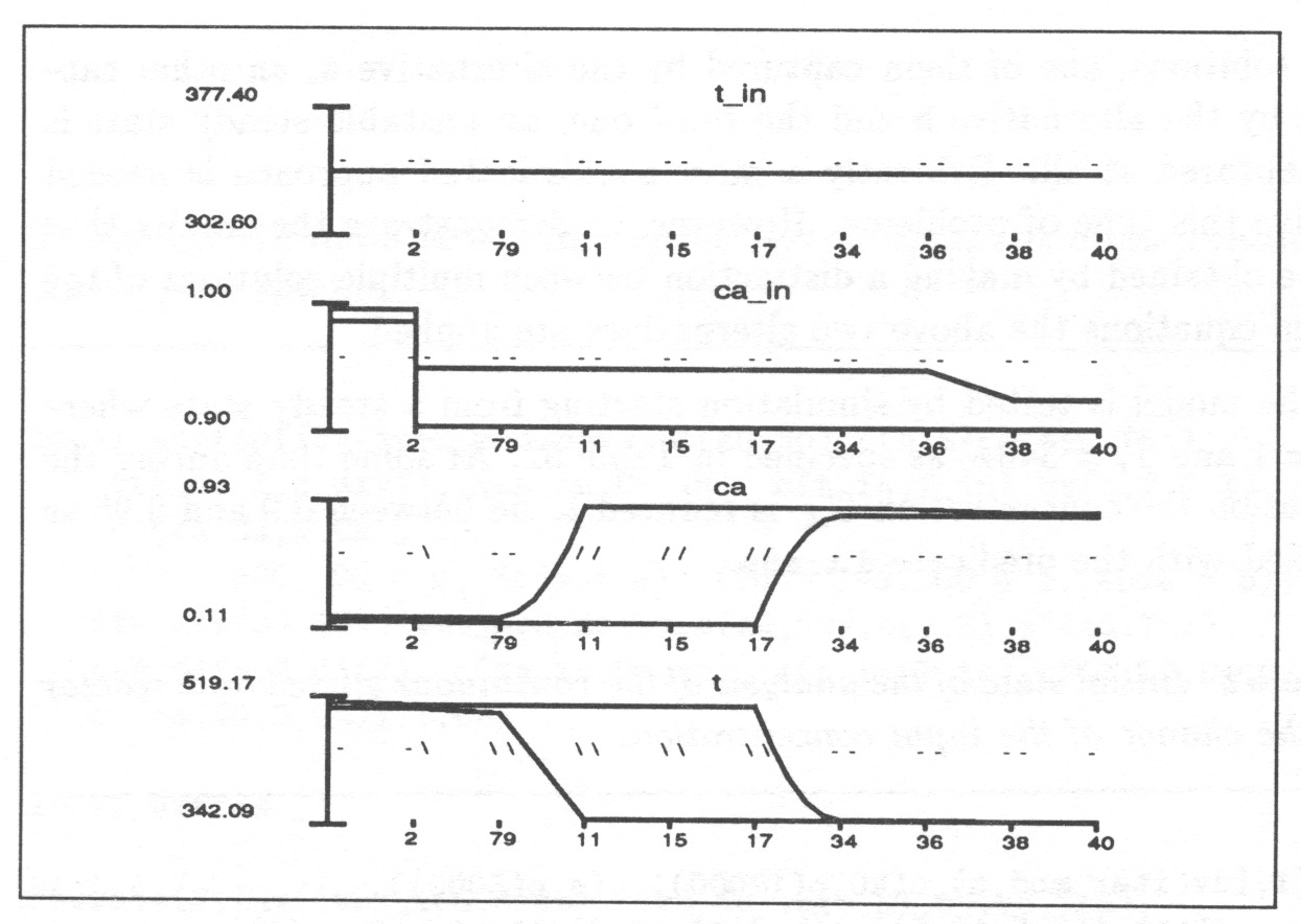
The prediction shows first a small decrease of concentration and then a large increase of it while the temperature decreases. It shows that the algorithm can tell the difference between the steady states and can capture the change of the steady state. The analysis indicates that in principle systems modelled with quite complicated equations can be handled successfully. However, it also reveals the need to further develop the algorithm.
7 OSCILLATING SYSTEMS
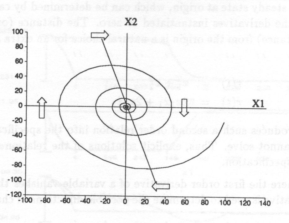
The systems examined this far have not had oscillating behaviour. When planning process plant automatics it can be often assumed, that the systems are overdamped by nature or there are feedback controllers which make them overdamped, so that no oscillating behaviour is observed. But of course this is not always the case. The analysis of oscillating behaviour is also a good test of the analysis algorithm.
The following simple linear second-order system is analyzed.
| (67) | |||||
| (68) |
The above equations alone are not sufficient for the ISIR-algorithm to tell a stable system from an unstable one. The explanation can be seen in Fig. 43. In principle the ISIR-algorithm considers the magnitudes of the state variables only on the lines in the drawing, where any of the variables or their derivatives vanish. Between the lines ISIR considers only the signs of the derivatives. This clearly is not sufficient to determine the stability of the system. In general numerical integration is needed to determine the exact trajectory. In this example integration would also be straightforward, because the model and its parameters are assumed to be known exactly.
However, it is possible to include additional constraint equations into the model to make the ISIR-analysis more accurate. In the current example the system has a steady state at origin, which can be determined by calling sys_eq with all the derivatives instantiated to zero. The distance (or the square of the distance) from the origin is a natural choice for an extra state variable.
| (69) | |||||
| (70) |
Equation 69 introduces such a second order relation into the specification which CLP() cannot solve. Thus, explicit solutions of the relation must be given in the specification.
At points where the first order derivative of a variable vanishes the second order derivative is used to determine the possible directions of change:
| (71) | |||||
| (72) |
Fig. 44 shows one of the resulting behaviours. The maximum distance from the origin decreases slowly. This is because the total energy is known to decrease. However, the minimum distance gets to zero very soon; during the first quarter of the revolution around origin. This is because the algorithm does not take into account the time elapsed in a state change and thus it is not known how much the energy can decrease during a state change.
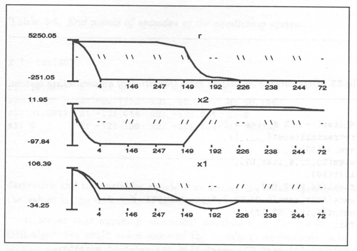
7.1 EMPLOYING NUMERICAL INTEGRATION
ISIR-algorithm represents the behaviour of a continuous time function as a — possibly branching — sequence of episodes. In Fig. 43 an episode is a segment of the curve during which neither of the derivatives change sign. In the previous section it was seen that if more accurate analysis is desired, time must be taken into account which again requires that the length of the path rather than only its endpoints must be considered. Thus, it is necessary to consider system state on different points in the path representing an episode. Table 53 shows how this can be accomplished with numerical methods to solve differential equations:
First sys_eq(X0) is called to tell the relations between state variables and their derivatives in the initial state. Then a simulation predicate is called to construct a set of equations telling the relations between the system states at N_iter time points. The initial state is (partially) instantiated with the call init(X0) and the final state is (partially) instantiated with the call final(Xf,F,DF_DT) where F tells the difference of the desired final state and the one given by the simulation. init_newt calls an iteration to search such a value for the integration time step DT which makes F zero.
tst(N_iter):-   % N_iter = 20,
    retractall(newt(_,_,_)),
    sys_eq(X0),!,
    simu(X0,Xf,N_iter,DT),
    init(X0),
    final(Xf,F,DF_DT),
    once(init_newt(0.01,DT,F,N_iter*DF_DT), F = 0),
    outpt(N_iter,DT,Xf),
    fail.

sys_eq([c(c1,C1),c(c2,C2),cv(x1,X1,D_X1),cv(x2,X2,D_X2)]):-
       D_X1 = X2,
       D_X2 = C1*X1 + C2*X2.

simu(Xa,Xf,N,DT):-
     sys_eq(Xb),
     integrate(Xa,Xb,DT),!,
     (N > 0 -> simu(Xb,Xf,N-1,DT) ; Xf = Xb).

integrate([],[],_).
integrate([H0|T0],[H1|T1],DT):-
     integ(H0,H1,DT), integrate(T0,T1,DT).

integ(c(Id,X),c(Id,X),_).
integ(u(Id,_), u(Id,_),_).
integ(cv(Id,X,DX), cv(Id,X1,DX1),DT):- X1-X = (DX+DX1)/2*DT.

init([c(c1,-1),c(c2,-0.25),cv(x1,X1,0),cv(x2,_,_)]):-
     X1 = 100; X1 = 150.

final([c(c1,C1),c(c2,C2),cv(x1,_,D_X1),cv(x2,_,F)],
      F, (C1*D_X1+C2*F)).
final([c(c1,_),c(c2,_),cv(x1,F,D_F),cv(x2,_,_)],F,D_F).
init gives two extreme values for X1. final specifies two alternatives; either the derivative of X2 vanishes or X1 becomes zero. Thus, init and final represent conditions which the ISIR-algorithm defines for the low level transitions predicates. Thus, the concept presented here can be directly integrated into the ISIR-algorithm.
A simple integration scheme integrate is applied. The predicate simu is called before any of the parameters — except the number of simulations steps N is given a value.
Newton iteration is applied to determine the time step of iteration that results to the desired final state. The iteration is implemented using assert and retract as on page 37 to allow iteration on backtracking which gives a clearer structure for the main program than the approach employed on page 50.
The result is shown in Table 54.
2 ?- tst(20).

x1: 20.8407  d: -83.363   x2: -83.363  d: 0
x1: 0        d: -80.7788  x2: -80.7788  d: 20.1947
x1: 31.2611  d: -125.044  x2: -125.044  d: 0
x1: 0        d: -121.168  x2: -121.168  d: 30.292
The above shows that it is possible to integrate numerical simulation in the ISIR-algorithm when necessary. In all the details the above is not sufficient. It is necessary to check that every point in the path satisfies the conditions of an episode: there should be no change of sign of any derivative and the variables should stay during the whole episode between the values in the endpoints of the episode.
It seems that applying numerical simulation at the low-level in the ISIR-algorithm could solve some of the problems encountered when analyzing systems having complicated continuous dynamics without losing the general problem solving power. However, some points require further consideration. For example, in the basic ISIR-algorithm it is sufficient to assume that external control is either increasing, decreasing or steady. When applying numerical simulation methods such an assumption results in heavy computation because constrained dynamic optimisation problems must be solved. Probably some simplifying assumptions and pre-analysis of the system equations are needed to achieve reasonable efficiency.
Summary
Analysis of an oscillating system reveals that considering only the endpoints of an episode and the direction of change during an episode results in quite vague predictions of the behaviour and in many superfluous predictions. The predictions can be pruned with additional constraints. However, it is also possible to apply numerical integration to determine the consistent state transitions.
8 DISCUSSION
Versatile solving of problems, many of which are quite abstract, is required in industrial process plant control. Theoretically the problem to be solved is to analyze/synthesize systems which are described partially with mathematical equations and inequalities, partially with logic clauses. Appropriate treatment of uncertainty is required so that it is not necessary to have highly accurate models to achieve dependable results. The main interest is on dynamic properties of hybrid systems, i.e. on developing methods for systems having both discrete-event and continuous-time dynamics.
Constraint logic programming language CLP() provides the ability to handle both logic clauses and mathematical equations and inequalities. It is only necessary to provide the solution mechanism for a certain type of non-linear equations and equations which do not have analytic solutions. This is done by programming explicit solutions for example for second order equations and using Newton iteration when it is not appropriate or possible to use explicit analytic solutions.
The full power of CLP() is not made use of. For example it is possible to dump into a string all the constraints attached to a variable or all the constraints in the model. This symbolic set of equations and inequalities can be easily manipulated using the Prolog pattern matching.
Uncertainty is represented as numeric intervals. Often interval problems are proposed to be solved iteratively applying some kind of local propagation. In ISIR the minimum and maximum of each variable is searched globally taking into account all the relevant equations simultaneously. The approach gives correct results contrary to sometimes proposed local propagation which may give only approximative results and sometimes even gives a result when there actually is none. The models required are also simpler because it is not necessary to use any interval operators when writing the models but ordinary equations are sufficient. The implementation technique is typical for constraint programming although may not have been applied before on solving interval problems.
Prolog is an appropriate tool to deal with discrete-event systems. In qualitative simulation continuous behaviour is considered a sequence of episodes separated by time points at which any of the derivatives of state variables change sign. Thus, implementing this principle of qualitative simulation in CLP() allows handling both discrete-event and continuous-time dynamics in a unified way. The representation of the behaviour is on an abstraction level required for example in designing discrete-event control systems.
The basic idea of specifying continuous-time behaviour as a set of transition constraints is adopted from QSIM but because quantitative knowledge is used it is possible to specify transitions directly from a time point to the next one.
Being restricted only to quantitative knowledge when modelling continuous-time systems has its pros and cons:
-
+
When a quantitative algorithm is constructed from the beginning it is possible to make more efficient use of quantitative information. Thus, many superfluous predictions can be avoided without missing any actual behaviours.
-
+
It is more straightforward to model systems where quantitative models are necessary to get any useful results.
-
-
In cases, where no quantitative knowledge is available, some quantitative information must be invented. This may lead to misleading results.
-
+
Because numeric landmarks are used, they are automatically shared among the state variables so that ordering of the landmarks of different variables is made use of. This helps to filter out some superfluous predictions. QSIM provides an option to specify the relative ordering of the landmarks of some of the variables.
-
-
The effect of shared landmarks is quite significant and it is introduced implicitly. For example specification tells nothing about the sign of . If then in one part of the specification an assignment is made and in a different part an assignment the sign of is determined maybe unintentionally.
In ISIR the actual landmarks are typically intervals rather than single values, but still the above applies.
-
-
It is not possible to specify a relation like m(X,Y) stating that Y is a monotonously increasing function of X. All the relationships must be represented as mathematical functions like for example . It is also possible to say that but and must be mathematical functions.
Inventing such functional relations with insufficient information on the actual system is annoying and may result in misleading results.
consists of programming, it is
computationally more be true.
8.1 FUTURE WORK
The ISIR-algorithm is a prototype for a kernel of a general problem solving tool. As a kernel only it requires additional modules to become a practical tool. In addition the previous examples indicate that there is need to improve the prototype. The following is a brief discussion on some possible improvements.
8.1.1 The basic algorithm
Complexity considerations
Constraint logic programming provides ways to reduce considerably the complexity of the computations compared to brute-force approach. These methods are made use of in the ISIR-algorithm. However, as a result it is impossible to estimate the complexity of the algorithm, because the complexity of the computation depends heavily on the system analyzed. Thus, the only way to estimate the complexity of practical problems is testing. The examples handled in this report are not extensive enough for this purpose.
No attention was paid on the complexity of the algorithm as long as the exemplary problems could be solved in a few minutes in a PC having a -486 25 MHZ processor and 16MB of core memory. So there is room for improvements of the efficiency. Currently it seems that more attention should be paid on space complexity than on time complexity.
It should be checked if any part of the basic algorithm introduces superfluous alternatives and thus causes unnecessary complexity. There are two sources of possible unnecessary alternatives:
-
•
The calls of the freeze-predicate are placed somewhat ad hoc in the code. Careful reconsideration of freezing the calls of predicates might reduce the complexity.
-
•
There may be unnecessarily many alternatives especially in the predicate which searches a point which satisfies given constraint equations inside a region. The more different alternatives are tried out, the more certain it is that a point is found when there is one. However, unnecessary alternatives heavily increase the complexity in cases when there is actually no solution. It should be straightforward to determine the minimum necessary set of alternatives to guarantee correct solution.
There are at least three different ways to implement the numerical iterations: Recursion with the variables instantiated, execution of the constraints once with uninstantiated variables and then recursive modification of the variables and finally use of backtracking instead of recursion. The complexity of the alternatives should be evaluated and the best one implemented.
There are also alternative ways to implement the main body of the algorithm. The space complexity of the alternatives should be evaluated. In addition in the current version states are stored unnecessarily in two places.
Solution of non-linear and non-analytic constraints
Non-linear constraints are treated with Newton iteration or with explicit solution formulas in a somewhat ad hoc manner. Which numeric method is most appropriate should be considered more carefully. There should be a more systematic way to make use of numeric iteration.
The method of solving two-point boundary value problems should be analyzed more carefully for accuracy.
Making use of existing numeric algorithms implemented in algorithmic programming languages like C should be considered.
Quantitative Temporal Information, Numerical Integration
The basic ISIR-algorithm does not give any information on the duration of the time intervals. In [missier] Missier and Travé-Massuyès discuss the possibilities to estimate the duration of time intervals in qualitative simulation. They present a method based on the second order Taylor formula for cases where some quantitative information on the system is available.
In Q3 discussed for example in [3] quantitative knowledge can be made use of when it is available to estimate the duration of episodes.
It was shown earlier that the state transitions can be determined with quantitative integration instead of the transition rules now used. This alternative should be implemented and the benefits, limitations and complications should be discussed and demonstrated in more detail.
If continuous state transitions are solved with numeric integration the temporal information can be obtained directly.
Hierarchical reasoning
A large system model consists of a hierarchy of modules where the modules often correspond to plant components and subsystems. It might be possible to apply higher and lower level models in reasoning. For example the state vector of a subsystem can be augmented with an extra variable telling if that subsystem is in operation or not, or a rough higher level model can be used to give rough limits for the values of some of the main variables and their directions of change. This can often reduce the search space a lot because there will be much less alternatives for the low level detailed models.
The current implementation forces all the variables to be always instantiated. In many cases only some of the variables are relevant. In principle it is possible to recursively go through the state transitions for a certain number of times and then instantiate the known variables and finally dump out the constraints attached to the interesting variables. This could reduce the complexity.
Symbolic landmarks, qualitative relations
ISIR is based on numeric landmarks only to allow easy implementation. As table 55 shows the symbolic computation needed in using symbolic landmarks can be implemented as a separate module without major modification of the existing algorithm. Of course implementation of such a module is a major effort.
symb_lm:-
% defining landmarks
   0 < Hx, 0 < Hy, 0 < Hz,
%  relations between landmarks
   Hx < Hy,
   Hx + Hy = Hz,
% values of  X, Y and Z
   0 < X, X < Hx,
   Y > Hy,
   0 < Z, Z < Hz,
%  add-constraint
   X + Y = Z,
   dump([X,Hx]),
   dump([Y,Hy]),
   dump([Z,Hz]).
1 ?- symb_lm.

0 < Hx
0 < X
X < Hx

Hy < Y
Y < 2*Hy
0 < Hy
0 < Y + Hy

Z < Hz
0 < Z
0.5*Hz < Z
0 < Hz
Currently ISIR does not allow the use of qualitative relations like for example mplus(y,x) requiring that y is a monotonously increasing function of x. However, it is possible to define a predicate like mplus(Y,X) which requires that the derivatives of X and Y have the same sign. Corresponding values can be handled in the same way. Hence it is possible to include in ISIR real qualitative simulation.
8.1.2 Describing the desired behaviour
The current version of ISIR can accomplish the low level tasks in action planning and control system design. The user should be provided means to specify the desired behaviour of the system to make it possible to solve higher level problems autonomously. A part of this specification are operational restrictions, which can be given as constraints that every state much satisfy. Operational restrictions can be specified easily in the ISIR framework. The goal state of a sequence of operations is also easy to specify. However, to be able to flexibly specify the desired behaviour it must be possible to specify also other types of characteristics. Currently ISIR provides many different ways to characterise the desired behaviour, but they require detailed knowledge of the implementation of ISIR.
The functional requirements of the system can be represented as a hierarchy of functions. Each function can be given preconditions which must be true before the function is allowed to be initiated. Support conditions tell what must be true during the execution of the function. Post-conditions finally tell what should be true after the execution of the function. Every function can be divided into a set of subfunctions. The lowest level functions as well as pre-, support, and post-conditions would have one-to-one correspondence with the system model.
8.1.3 Supporting the model generation
One of the motivations for developing ISIR is to help control system designers to cope with the complexity of the design and help them to modify the control system to reflect the changes in the design of the plant. To achieve this modelling and remodelling of the plant should be fast and simple.
The principles of how to support modelling have been presented but no general-purpose tool is implemented. Because databases of existing CAD-tools should be used extensively a flexible interface should be provided. Defining an intermediate language and providing transformation from it to ISIR-models could be the best choice. The intermediate language should be defined so that existing CAD-tools can easily produce models in it.
8.1.4 Applications
Qualitative reasoning and constraint logic programming provide many already implemented techniques and tools which can be applied on solving real-life problems. However, much of the later research and development seems to be triggered by difficulties encountered when trying to solve practical problems with the original principles of qualitative modelling. It seems that the principles are sound but not sufficient for solving but a limited set of practical problems. On the other hand for example the development of Q3 shows that the original principles of qualitative modelling can be successfully complemented in many ways.
Much of the latest development has been made use of also when implementing ISIR but the previous sections on future work reveal that there are still many things to be tried out. Two mistakes can be made at this phase:
-
•
A lot of time and resources will be spent on a universal stand-alone tool with very sophisticated user-interface etc. There will be demonstrations but the risk is that they are not selected to represent practical problems but the properties of the tool so that actually only very few real-life problems can be solved with the tool.
-
•
A particular real-life problem may be chosen to be solved with qualitative modelling. A large complex problem requires a lot of routine work leaving less time for the development of the generic techniques and tools required for that type of problems. Instead, quick and dirty fixes are made to get the tool work in time. Instead of achieving a generic tool a messy procedure capable of solving only the very particular problem is produced.
Thus, careful compromising is needed.
Because new challenges are rising and because qualitative reasoning is becoming mature enough to meet those challenges, future research should be directed towards solving practical problems. Problems on various restricted domains not solvable with existing methods should be attacked.
-
•
An area with practical significance and problems seemingly solvable by qualitative reasoning should be selected.
-
•
Qualitative reasoning and all the other techniques and tools should be forgotten. Real-life problems never map one-to-one on theoretical methods.
-
•
The application area must be analyzed to give a formal representation of the problems to be solved. The problems difficult to give formal representation are also difficult to solve with computerised tools. The man-machine interface should be somewhere in the region where the problem formulation turns from formal to informal.
-
•
The problems must be analyzed to choose the techniques to solve them. To some extent different types of subproblems can be solved separately with existing tools but major breakthroughs require tight integration of different techniques. An example on such successful tight integration is CLP(), where resolution and linear programming are integrated seamlessly.
-
•
The software to solve the problems should be specified to the extent that shows that the software is possible to implement and that allows the estimation of the effort needed to implement it. Existing tools and proof-of-the-principle prototypes must be used to demonstrate possible implementations of the crucial and theoretically most demanding parts3030The underlying objective of the development of the ISIR-tool has been to test and demonstrate that the crucial parts of a tool to support design and verification of process plant automatics can be implemented..
-
•
In addition to using end-users when analyzing the problem domain also demonstrating the principles of the planned solution to them might fertilize ideas of new applications.
-
•
The development of the tool must be considered a rapid prototyping project, which requires careful consideration of the quality of the software because there will be a lot of minor and major modifications of the program. A high-level programming language which is used to implement the software is often used also as an executable specification language and the code itself must also often serve as its own documentation. It should be easy for any experienced programmer to understand and to modify the code. Configuration control requires special attention when alternative solutions are tried out. Verification and validation must also be paid special attention: When the product is experiencing and on-going evolution, verification and validation must also be an on-going process to reveal as soon as possible any deviations from the requirements. At the same time verification and validation should interfere with the development work as little as possible.
9 CONCLUSIONS
The difficulty to realize the full behaviour of complex systems causes errors in control system design and plant operation especially in abnormal situations. There are too many things that may occur and too many complex relationships for a human mind to make the synthesis of them. The usefulness of simulation is a good evidence of this, although simulation provides only one kind of synthesis of the available knowledge.
The main potential benefits of computerised tools in tasks related to plant control and operation are the improved efficiency, better coverage of different situations and more dependable accomplishment of many routine tasks. Functional design of control systems, action planning, fault diagnosis and functional verification of control and monitoring systems are some potential applications of knowledge-based tools.
Most of the knowledge required to accomplish such tasks can be obtained from plant documentation and from general laws of physics and the knowledge can be represented as a plant model. Such deep knowledge can be elicitated systematically, partially even automatically, and the knowledge-base can be made comprehensible and thus easy to validate. Heuristics should be minimised and used only when its effect on the solution is evident.
Making efficient use of computers in various tasks related to process plant control and operation requires
-
•
Versatile problem solving based on the plant model constructed from mathematical equations and logic clauses.
Flexible problem solving is important because of the large variety of the type of problems encountered. Deep knowledge and model-based reasoning are the best way to construct a dependable system for flexible problem solving. The knowledge representation formalism must be flexible enough to allow the use of both mathematical equations and inequalities and clauses of first order logic.
-
•
Proper handling of systems having both continuous and discrete dynamics.
There are both discrete and continuous control inputs and measurements. Sometimes a part of the plant is convenient to model to have discrete dynamics and some control functions are implemented as discrete-event systems. But still significant parts of plants have continuous-time dynamics.
-
•
Knowledge representation on an abstraction level higher than real-valued functions.
One trajectory showing the step response is sufficient to tell the essential properties of a feedback controller of a linear system. For non-linear systems controlled with a discrete-event system this is not the case. Usually a small number of trajectories would cover all the significantly different cases, but those trajectories cannot be identified. This is because the essential characteristics are represented on a higher abstraction level.
-
•
Proper handling of uncertainty and incompleteness.
Neither the plant models nor the operational requirements can be specified accurately and completely.
Many of the principles of qualitative simulation can be applied when implementing model-based reasoning. The one directly visible is to represent system behaviour as a (branching) sequence of episodes separated by significant time points. During an episode none of the derivatives of the system state variables change sign. Significant time points mark instances at which the derivatives change sign, some threshold value is exceeded, or some discrete state variable gets a new value.
On the domain of industrial process plants numeric intervals are an appropriate knowledge representation type. Plant models, initial and goal states etc. can be represented by giving the constants and the state variables values which are intervals rather than single values. As a result plant behaviour is represented as episodes characterised by upper and lower limits of the magnitudes of the variables and by the signs of the first derivatives at initial and final time. Such a representation is useful in many reasoning tasks.
Modern methods of knowledge-based systems have the necessary properties to implement a tool satisfying the above requirements. Logic programming makes it possible to solve in practice many problems which — if tried to be solved by procedural programming languages — result in an overwhelming set of if-then-else clauses. Constraint logic programming languages — like CLP() — extend logic programming to solving also mathematical equations and inequalities.
The ISIR-algorithm developed in this work is a prototype kernel for model-based reasoning used to develop and validate principles of model-based reasoning. Flexible use of model-based reasoning requires in addition computerised support for model generation.
ISIR shows that it is possible to achieve many significant properties of qualitative reasoning even when using purely quantitative models of continuous-time subprocesses. Allowing only quantitative knowledge restricts the domain of application but allows efficient use of numerical methods, which improves the problem solving capabilities in that restricted domain.
There are two communities working on continuous time systems: those representing traditional simulation and control engineering and those working on artificial intelligence. Although they have different goals they still could benefit from each other. Both communities have methods which the others should know as well. AI community sometimes lacks the basic understanding of continuous-time dynamic systems while they have fresh ideas on what kind of problems will be encountered in the future.
In addition to the above the analysis and synthesis of discrete-event and continuous-time dynamic systems are still very different worlds. The results show that unifying these different approaches by implementing principles of qualitative reasoning in constraint logic programming is possible.
References
- 1 Baehr, H. D. Thermodynamik. Springer Verlag, Berlin/Göttingen/Heidelberg, 1962.
- 2 D. Berleant, B. Kuipers. Bridging the gap from Qualitative to Numerical Simulation. Artificial Intelligence Laboratory, The University of Texas, March 1991 AI 91-158
- 3 D. Berleant, B. Kuipers. Qualitative and Quantitative Simulation: Bridging the gap from. September 1992.
- 4 S. Bologna, T. Sivertsen, H. Välisuo. Rigorous Engineering Practice and Formal Reasoning of Deep Domain Knowledge — The Basis of Dependable Knowledge Based Systems for Process Plant Control. International Journal of Software Engineering and Knowledge Engineering. Vol. 3, No. 1(1993) 53-98. World Scientific Publishing Company.
- 5 F. E.Cellier, N. Roddier. Qualitative State Spaces: A Formalization of the Naive Physics Approach to Knowledge-Based Reasoning. Proceedings of the Second Annual Conference on AI, Simulation and Planning in High Autonomy Systems. Theme: Integrating Qualitative and Quantitative System Knowledge, Cocoa Beach, FL, USA 1-2 April 1991 (Los Alamitos, CA, USA: IEEE Comput. Soc. Press 1991).
- 6 Challenges to Control: A collective View. Report of the Workshop held at the University of Santa Clara on September 18-19 1986. IEEE Transactions on Automatic Control Vol. AC-32 No. 4 April 1987.
- 7 W.F. Clocksin, C.S. Mellish. Programming in Prolog. Springer-Verlag, Berlin, Heidelberg, New York. (1981).
- 8 William Clocksin. Defining Digital Circuits with Prolog. Byte, August 1987.
- 9 J. Cohen. Constraint logic programming languages. Communications of the ACM, Vol. 33, No. 7, July 1990.
- 10 A. Colmerauer. An Introduction to Prolog III. Communications of the ACM, July 1990, Vol. 33, No. 7.
- 11 D.T. Dalle Molle. Qualitative Simulation of Dynamic Chemical Processes, Ph.D. Dissertation, Department of Chemical Engineering, University of Texas at Austin, TX(1989).
- 12 A.B. Dobrzeniecki, L.M. Lidsky. Modeling and Analysis of Complex Physical Systems Using Model-Based Reasoning with Constraint Satisfaction. Proceedings of the 7th. Power Plant Dynamics, Control and Testing Symposium, Knoxville, TN, USA, 15-17 May 1989.
- 13 Folkert Dokter. Steuerung von Chargenprozessen mit wechselnden Rezepturen. Automatisierungstechnische Praxis 33 (1991).
- 14 F. Cheriaux, J. Ancelin. Expert Systems Monitoring in a Nuclear Power Plant: A living Example and Prospects at EdF. Expert systems in the nuclear industry. IAEA-tecdoc-660, July 1992.
- 15 D. L. Dvorak. Monitoring and Diagnosis of Continuous Dynamic Systems using Semiquantitative Simulation. Doctoral Dissertation. The University of Texas at Austin. (1992).
- 16 A. Farquhar, B. Kuipers, J. Rickel, D. Throop et al. QSIM: The program and its use. Department of Computer Sciences, University of Texas at Austin, Austin, Texas 78712 USA (kuiperscs.utexas.edu) (1992).
- 17 Kenneth D. Forbus. Qualitative Process Theory. Artificial Intelligence 24, 1984.
- 18 P.Fouché, B. J. Kuipers. Reasoning About Energy in Qualitative Simulation. IEEE Transactions on Systems, Man and Cybernetics, Vol. 22, No. 1. January/February 1992.
- 19 P. Fouche. Towards a Unified Framework for Qualitative Simulation, Ph.D. Dissertation, University of Compiègne, 1992.
- 20 J. Fox. Decision theory and autonomous systems. Decision Support Systems and Qualitative Reasoning. M.G. Singh and L. Trace-Massuyès (eds.). Elsevier Science Publishers B.V. (North Holland). 1991.
- 21 J. G. Gleary. Logical Arithmetic. Future Computing Systems, Vol. 2. Number 2. 1987.
- 22 Harel, D. Dynamic logic. In Handbook of Philosophical Logic, Volume II: Extensions of Classical Logic, D. Gabbay and F. Guenthner, Eds., D. Reidel Publishing Company, Dordrecht, 1984, pp. 497–604.
- 23 Heintze, N. Jaffar, J., Michaylov S., Stuckey S., Yap, R. The CLP()Programmer’s Manual, Version 1.1., 1991. IBM Thomas J Watson Research Center, PO Box 704, Yorktown Heights, NY 10598, U.S.A.
- 24 IEC 848. Preparation of Function Charts for Control Systems, 1988. International Electrotechnical Commission.
- 25 J.R. James. Future of Intelligent Control Systems. Instrumentation, Controls and Automation in Power Industry. Vol. 34 Proceedings of the Thirty-Fourth Power Instrumentation Symposium, St. Petersburg Beach, FL, USA, 3-5 June 1991.
- 26 M.E. Janusz, V. Venkatasubramanian. Automatic Generation of Qualitative Descriptions of Process Trends for Fault Detection and Diagnosis. Engineering Applications of Artificial Intelligence, Vol. 4, No. 5, 1991.
- 27 A-E. Johansson, A. Eriksson-Granskog, A. Edman. En match med Prolog. Studentlitteratur, Lund, Sweden. (1985)
- 28 H. Kay, B. Kuipers. Numerical Behaviour Envelopes for Qualitative Models. June 1992.
- 29 J. De Kleer, J. S. Brown. A Qualitative Physics Based on Confluences. Artificial Intelligence 24, 1984.
- 30 G. G. Koch. Modular Reasoning — A new Approach towards Intelligent Control. Diss. ETH No. 10105. Swiss Federal Institute of Technology. Zürich 1993.
- 31 Kuipers, B. Qualitative Simulation. Artificial Intelligence, Vol. 29, pp. 289-338
- 32 Kuipers, B. and Berleant D. Using incomplete quantitative knowledge in Qualitative Reasoning. Proc. nat. Conf. on Artificial intelligence (AAAI-88), 1988. Morgan Kaufmann, Los Altos, California.
- 33 Kuipers, B. Qualitative Reasoning: Modelling and Simulation with Incomplete Knowledge. Automatica, Vol. 25, No. 4, 1989.
- 34 B. Kuipers. Higher-order derivative constraints in qualitative simulation. Artificial Intelligence 51 (1991). Elsevier.
- 35 Catherine Lassez. Constraint Logic Programming. Byte, August 1987.
- 36 Lee, W.W., Chiu, C. and Kuipers B. Developments Towards Constraining Qualitative Simulation. Ai TR87- 44 January 1987. Artificial Intelligence Laboratory, The University of Texas at Austin.
- 37 Leitch, R.R. Modelling of Complex Dynamic Systems. IEEE Proceedings, Vol. 134, Pt. D, No. 4, July 1987.
- 38 Nancy Leveson. The Challenge of Building Process-Control Software. IEEE Software, November 1990.
- 39 A.G.J. MacFarlane, G. Gruebel, J. Ackermann. Future Design environments for Control Engineering.
- 40 Louise Travé-Massuyes. Qualitative Reasoning from Different Aspects and Potential Applications to Decision Support Systems. Decision Support Systems and Qualitative Reasoning. M.G. Singh and L. Trace-Massuyès (eds.). Elsevier Science Publishers B.V. (North Holland). 1991.
- 41 R. Milne. Strategies f Information in Qualitative Simulation. Proceedings of the Second Annual Conference on AI, Simulation and Planning in High Autonomy Systems. Theme: Integrating Qualitative and Quantitative System Knowledge, Cocoa Beach, FL, USA 1-2 April 1991 (Los Alamitos, CA, USA: IEEE Comput. Soc. Press 1991).
- 42 J. S. Ostroff, W.M. Wonham. A Framework for Real-Time Discrete Event Control. !!! Where ????
- 43 Price, C.and M. Lee. Applications of deep knowledge. Artificial Intelligence in Engineering, 1988, Vol. 3, No. 1
- 44 Raiman, O. Order of Magnitude Reasoning. Proceedings of the National Conference on Artificial Intelligence, American Association for Artificial Intelligence, 1986.
- 45 P.J. Ramadge and W.M. Wonham. Supervisory control of a Class of Discrete Event Processes. Siam J. Control and Optimization. Vol 25, No 1, January 1987.
- 46 Sacks, E. Piecewise linear reasoning. Proc. Nat. Conf. on Artificial Intelligence (AAAI-87). Morgan Kaufmann, Los Altos, California.
- 47 Sacks, E. Hierarchical reasoning about inequalities. Proc. Nat. Conf. on Artificial Intelligence (AAAI-87). Morgan Kaufmann, Los Altos, California.
- 48 E. Sacks. A dynamic System Perspective on Qualitative Simulation. Artificial Intelligence 42 (1990).
- 49 Shoham, Y. Ten Requirements for a Theory of Change. New Generation Computing, 3 (1985).
- 50 Stephanopoulos. The future of Expert Systems in Chemical Engineering. Chemical Engineering Progress Vol. 85 no. 9, September 1987.
- 51 Tuominen, H. Elementary Net Systems and Dynamic Logic. In Advances in Petri Nets 1989, G. Rozenberg, Ed., Springer-Verlag, Berlin, 1990, pp. 453–466.
- 52 Valisuo, H. Qualitative Modelling in Process Plant Control and Operation. OECD Halden Reactor Project, HWR-295, May 1991. Halden, Norway.
- 53 Heikki Valisuo. Model-Based Reasoning in the Design of Discrete-Event Control. Proceedings of ”New Directions in Artificial Intelligence”, Otaniemi, Finland, 9.-11.6.1992. Finnish Artificial Intelligence Society.
- 54 A study of Terminology and issues in Qualitative Simulation. Simulation, January 1989
- 55 W.M.Wonham. Some Remarks on Control and Computer Science. IEEE Control Systems Magazine. April 1987.
- 56 H. Voss. Representing and Analyzing Causal, Temporal, and Hierarchical Relations of Devices. SEKI Report SR-87-17 (Doctoral Thesis), Fachbereich Informatik, Universität Kaiserslautern, 1986.
- 57 L. A. Zadeh. Fuzzy Logic. Computer, April 1988.
Appendix A ABOUT PROLOG
The following is not a general introduction to Prolog, but it introduces the features of Prolog which are necessary for reading this document.
A.1 VARIABLES
Prolog variables are strings starting with a capital letter. Other strings in the program are atoms3131In these examples it is like that. The Prolog syntax allows some other strings to be variables as well. The variables in Prolog programs may be instantiated or uninstantiated. An instantiated variable has obtained an atomic value, while an uninstantiated one has not.
f(1, one).
f(2, two).
f(_, too_big).
A ‘number-to-symbol’-conversion predicate f is defined.
1, 2,
one, two and too_big are atoms (‘constants’) and ‘_’ is
a
special ‘dont́ care’-variable.
| ?- f(1,one).
yes
| ?- f(1,two).
no
f(X,Y) is true if X and Y are defined to be in
relation
f, and false otherwise.
| ?- f(1,S). S = one | ?- f(N,two). N = 2 |
Calling f(X,Y) also tells which values X and Y must be assigned to satisfy the relation. |
| ?- f(4,S). S = too_big | ?- f(N,four). no |
too_big is in relation with ‘_’, i.e it is in relation with anything. On the contrary four is not defined to be in relation f at all. |
Table 56 is an example on defining the relation between numbers and corresponding strings. Queries can be made to find out if certain atoms are in the relation. If there are variables in the queries, it is checked, if the variables can be replaced by some atoms so that they satisfy the relation. Note that there is neither input nor output: Prolog predicates define relations, not functions.
Prolog is an untyped language. Thus, with the same member-predicate it is possible to check if and if pair(a,D) {pair(x,y), pair(b,c), pair(a,b)}. In CLP() some distinction must be made between numeric variables and others. In addition in CLP() it is possible to have partially constrained numeric variables.
There are meta-level predicates which tell if the variable is instantiated or not. In programming they are needed only when making some special constructions. Table 57 demonstrates the instantiation of the variables and applies such meta-level predicates.
pr(X):- ground(X),
    printf('% is ground\n',[X]).
pr(X):- arithmetic(X),
    dump([X],[x],C),
    printf('% is an arithmetic term constrained by %\n',[X,C]).
pr(X):- functor(X),
    printf('% is an ungrounded construct\n',[X]).
pr(X):- printf('% is unconstrained\n',[X]).

1 ?- pr(X), X < 5, pr(X), X > 0, pr(X), X = 3, pr(X).
_h1 is unconstrained
_t1 is an arithmetic term constrained by [x < 5]
_t1 is an arithmetic term constrained by [^-(x) < 0, x < 5]
3 is ground

2 ?- pr(X), X = pair(A,B), pr(X), B = b, pr(X), A = a ,pr(X).
_h1 is unconstrained
pair(_h4, _h5) is an ungrounded construct
pair(_h4, b) is an ungrounded construct
pair(a, b) is ground
A.2 FACTS AND RELATIONS
Facts and relations can be defined as in Table 58. mother(Mother, Child) tells a relation between two persons.
mother(eeva,maija).
mother(eeva,kaisa).
mother(kaisa,anni).
mother(kaisa,riikka).
mother(maija,annastiina).
mother(maija,ilona).
mother(liisa,heikki).
mother(helka,jussi).
mother(helka,olli).
father(olli,monna).
grand_mother(X,Z):- mother(X,Y), mother(Y,Z).
grand_mother(X,Z):- mother(X,Y), father(Y,Z).
parent(A,B):- mother(A,B).
parent(A,B):- father(A,B).
cousin(A,B):-
      dif(X,Y),
      parent(X,A), parent(Z,X),
      parent(Z,Y), parent(Y,B).
The relations can be connected to one another. The program in Table 59 can be interpreted roughly as “if there are X, Y and Z so that X is Y’s mother and Y is Z’s mother then X is Z’s grandmother”. The second line introduces another alternative for X being Z’s grandmother.
[8] demonstrates Prolog with some examples on digital circuits. Fig. 45 shows XOR-function implemented with nand-circuits. Nand-circuit and xor-function can be specified in Prolog. Then, it can be searched for example what the output for given input values is, what the other input must be if the other input is known and the desired output is given, or which inputs give a given desired output as shown in Table 60.
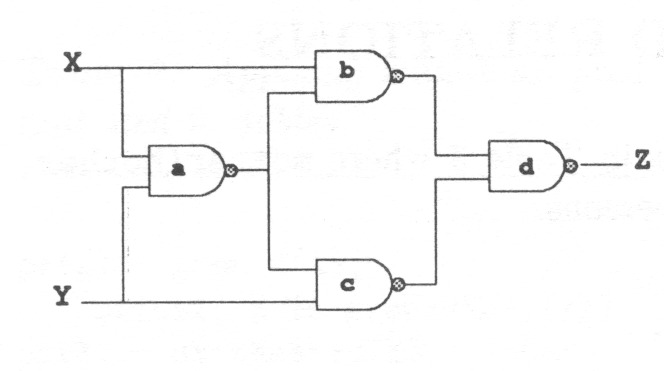
nand(0,0,1).
nand(0,1,1).
nand(1,0,1).
nand(1,1,0).
xor(X,Y,Z):-
    nand(X,Y,A),
    nand(X,A,B),
    nand(Y,A,C),
    nand(B,C,Z).
| ?- xor(0,1,X).
X = 1 ? ;
no

| ?- xor(X,0,Y).
X = 0, Y = 0 ? ;
X = 1, Y = 1 ? ;
no
|
| ?- xor(X,Y,1). X = 0, Y = 1 ? ; X = 1, Y = 0 ? ; no |
A.3 BACKTRACKING
Backtracking is central for Prolog execution. Prolog interpreter uses it to find a fact or a relation that satisfies the goal. Table 61 shows a trace of execution of a Prolog program with a lot of backtracking. When a goal fails, a previous goal is checked for any alternatives. This is done until a goal with untried alternatives is found. Such a goal is redone and the execution then proceedes forward.
backtracking:-
    mother(Mother,Child),
    Child = jussi.

?- backtracking.
1 1 Call: backtracking
2 2 Call: mother(_177,_178)
2 2 Exit: mother(eeva,maija)
3 2 Call: maija=jussi
3 2 Fail: maija=jussi
2 2 Redo: mother(eeva,maija)
2 2 Exit: mother(eeva,kaisa)
3 2 Call: kaisa=jussi
3 2 Fail: kaisa=jussi
2 2 Redo: mother(eeva,kaisa)
2 2 Exit: mother(kaisa,anni)
3 2 Call: anni=jussi
3 2 Fail: anni=jussi
2 2 Redo: mother(kaisa,anni)
2 2 Exit: mother(kaisa,riikka)
3 2 Call: riikka=jussi
3 2 Fail: riikka=jussi
2 2 Redo: mother(kaisa,riikka)
2 2 Exit: mother(maija,annastiina)
3 2 Call: annastiina=jussi
3 2 Fail: annastiina=jussi
2 2 Redo: mother(maija,annastiina)
2 2 Exit: mother(maija,ilona)
3 2 Call: ilona=jussi
3 2 Fail: ilona=jussi
2 2 Redo: mother(maija,ilona)
2 2 Exit: mother(liisa,heikki)
3 2 Call: heikki=jussi
3 2 Fail: heikki=jussi
2 2 Redo: mother(liisa,heikki)
2 2 Exit: mother(helka,jussi)
3 2 Call: jussi=jussi
3 2 Exit: jussi=jussi
1 1 Exit: backtracking
A.4 RECURSION AND LISTS
Items separated with commas and included in brackets form a Prolog list, which can be considered as an ordered set.
Recursion is commonly used in Prolog programs, the member-predicate in Table 62 being a typical example. [H|T] stands for a list whose first item is H, and T is the rest of the list. X is a member of the list if it is equal to the first item in the list or if it is a member of the rest of the list.
| ?- [a,b,c,d,e,f] = [H|T].
H = a,
T = [b,c,d,e,f]

member(X,[X|_]).
member(X,[_|T]):-
	member(X,T).

| ?- member(e,[a,b,c,d,e,f]).
yes

| ?- member(c,[a,b,e,f,h]).
no
| ?- member(X,[a,b,c]).
X = a ? ;
X = b ? ;
X = c ? ;

| ?- member(a,X).
X = [a|_72] ? ;
X = [_71,a|_78] ? ;
X = [_71,_77,a|_84] ?
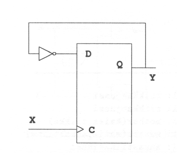
In Fig. 46 there is a divide-by-2 frequency divider taken from the example in [8]. Because it is an example of sequential logic it can be used to illustrate the use of Prolog in analyzing dynamic systems. The divider is constructed of a flip-flop and an inverter. The next state Q_next of the flip-flop depends on the current state Q and the data input D. The flip-flop is triggered by (rising edge of) the signal C. The input sequence is represented as a list of 1’s and 0’s. Predicate div in Table 63 specifies the circuit and predicate divide is used to ‘simulate’ the circuit. It recurs through the input list and produces the corresponding output list.
inv(0,1).
inv(1,0).

% dff(D,C,Q,Q_next).
dff(1,0,1,1).
dff(1,0,0,0).
dff(0,0,1,1).
dff(0,0,0,0).
dff(1,1,1,1).
dff(1,1,0,1).
dff(0,1,1,0).
dff(0,1,0,0).
div(X,Q,Y):-
     inv(Q,D), dff(D,X,Q,Y).

divide([],Q,[]).
divide([X|Xs],Q,[Y|Ys]):-
    div(X,Q,Y),
    divide(Xs,Y,Ys).

| ?- divide([1,1,1,1,1,1],0,Y).
Y = [1,0,1,0,1,0]

| ?- divide([0,1,0,0,1,1,0,0],0,Y).
Y = [0,1,1,1,0,1,1,1]
A.5 OTHER STRUCTURES - A BINARY TREE
Different structures can be represented as Prolog facts. For example a binary tree can be specified as a set of relations between a node and its left and right subtree as node(Node,Left, Right).
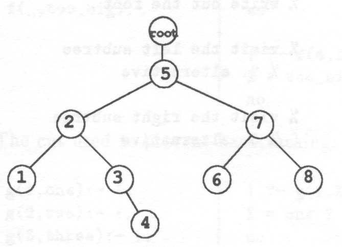
‘Generate-and-fail’ approach can be applied for example when Prolog is used in writing programs. Prolog first tries one of the alternatives and if it fails it backtracks to the previous point where there are other alternatives and chooses the next alternative. Using ‘fail’-predicate appropriately makes all the alternatives fail at the end thus forcing Prolog to try out all of them. Table 64 shows a generate-and-fail program to visit the nodes of a binary tree.
Because the predicate in Table 64 finally always fails, only its side-effects — in this case the text written on the terminal or in a file — can be made use of. The only reason to make a program like that is that it is easy to code and efficient to run.
In this case a more general program is as simple to code, see Table 65.
tree_visit1(Node):-                    % 1. alternative
      format(' tree(~w',[Node]),     % write out the root
      node(Node,Left,Right),
      tree_visit1(Left).             % visit the left subtree
tree_visit1(Node):-                    % 2. alternative
      node(Node,Left,Right),
      tree_visit1(Right).            % visit the right subtree
tree_visit1(Node):-                    % 3. alternative
       write(')'),
       fail.
The output is the following:
| ?- tree_visit1(root).
 tree(root tree(5 tree(2 tree(1) tree(3 tree(nil) tree(4)))
         tree(7 tree(6) tree(8))) tree(nil))
no
tree_visit2(Node,tree(Node,LTree,RTree)):-
      node(Node,Left,Right),
      tree_visit2(Left,LTree),
      tree_visit2(Right,RTree).
tree_visit2(Node,Node).
Giving the result as an argument.
| ?- tree_visit2(root,Tree).
Tree =
tree(root,tree(5,tree(2,1,tree(3,nil,4)),tree(7,6,8)),nil) ?
yes
| ?-
A.6 THE ‘CUT’
The ‘cut’, ‘!’ causes many complications and should be used with special care. ‘cut’ prevents Prolog from trying other alternatives after one of the alternatives has succeeded. Table 66 shows the behaviour of the same program with and without the cut.
All the alternatives:
f(1,one).
f(2,two).
f(3,three).
f(_,too_big).
|
| ?- f(1,X). X = one ? ; X = too_big ? ; no | ?- f(4,X). X = too_big ? ; no |
The cut used to prevent backtracking:
g(1,one):- !.
g(2,two):- !.
g(3,three):- !.
g(_,too_big).
|
| ?- g(1,X). X = one ? ; no | ?- g(4,X). X = too_big ? ; no |
A.7 METALOGICAL FEATURES
Metalogical features cannot be represented with predicate logic contrary to basic Prolog constructs. The ‘cut’ is a metalogical feature. All side-effects are also metalogical features. One of the ways to produce side-effects is to use assert- and retract-commands. After assert(p(a,b))-command calling p(a,b) succeeds, i.e. the predicate p(a,b) is added into the program. retract(p(a,b)) removes the predicate p(a,b). assert and retract can be used to pass parameters outside the parameter lists or even to modify the program during execution, which must be avoided.
However, assert and retract can also be used to integrate a data-base in a Prolog program. If assert and retract are used only in modifying a data-base separate from the program body, then their use is acceptable.
In the ISIR-algorithm assert is used to only one purpose, to implement a sort of ‘findall’ predicate shown in Table 67. can be determined by the program in Table 67.
a(0). a(1). a(-5). a(3).
b(0). b(3). b(5). b(-3).

limit:-
        retractall(ab(_,_)), % clean up
        a(A), b(B),
        Z is A+B,
        0 < Z, Z < 5,        % inside the limits
        assert(ab(A,B)),     % memorise
        fail.                % force backtracking for other
                             % alternatives
Now all the acceptable ab(A,B) are asserted.
| ?- limit.
no
| ?- ab(A,B).
A = 0, B = 3 ? ;
A = 1, B = 0 ? ;
A = 1, B = 3 ? ;
A = 3, B = 0 ? ;
no
| ?-
Some dialects of Prolog have a findall command which does the same job as the above program, see Table 68.
all(X):- findall(ab(A,B),limit(A,B),X).

limit(A,B):-
        a(A), b(B),
        Z is A+B,
        0 < Z, Z < 5.

| ?- all(X).
X = [ab(0,3),ab(1,0),ab(1,3),ab(3,0)] ?
A.8 CONSTRAINT LOGIC PROGRAMMING
Constraint logic programming can be seen as an extension of Prolog. The Prolog interpreter tries out the different alternatives provided by the program to find for the variables such a combination of values which satisfies the goal. In ordinary Prolog it is not possible to state that two uninstantiated variables must be instantiated to different values. Thus, for example the testing of inequality must be accomplished only after the variables get instantiated. Prolog-II provides a diff-predicate, which handles properly this problem. In constraint logic programming it is possible to constrain the allowable set of instantiations of a variable more generally in advance.
Constraint logic programming languages like Prolog-III and CLP() allow the use of mathematical equations and inequalities as constraints. [23] gives examples on CLP(), see Table 69.
fib(0, 1).
fib(1, 1).
fib(N, X1 + X2) :-
      N > 1,
      fib(N - 1, X1),
      fib(N - 2, X2).
4 ?- fib(14,F).
F = 610

5 ?- fib(N,610).
N = 14

6 ?- F > 7, F < 9, fib(N,F).
N = 5, F = 8
In [35] Lassez demonstrates CLP(). The task is to connect two resistors (R1 and R2) in Fig. 48 in series with a cell (V) so that the voltage over R2 is The available resistors are , , and and the available cells 10V and 20V. The solution to the problem is shown in Table 70.
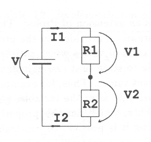
ohmlaw(V, I, R):-
	V = I * R.

kirchoff(L):-
	sum(L, 0).

sum([], 0).
sum([H | T], N):-
    H + M = N,
    sum(T, M).
availres(10).
availres(14).
availres(27).
availres(60).
availres(100).

availcell(10).
availcell(20).
2 ?- 14.5 < V2, V2 < 16.25, availres(R1), availres(R2),
     availcell(V), ohmlaw(V1,I1,R1), ohmlaw(V2,I2,R2),
     kirchoff([I1,-I2]), kirchoff([-V,V1,V2]).
I2 = 0.54054 I1 = 0.54054 V1 = 5.4054 V = 20 R2 = 27 R1 = 10 V2 = 14.5946 *** Retry? y |
I2 = 0.27027 I1 = 0.27027 V1 = 3.78378 V = 20 R2 = 60 R1 = 14 V2 = 16.2162 *** Retry? y |
I2 = 0.15748 I1 = 0.15748 V1 = 4.25197 V = 20 R2 = 100 R1 = 27 V2 = 15.748 |